「机器学习-李宏毅」:HW2-Binary Income Predicting
这篇文章中,手刻实现了「机器学习-李宏毅」的HW2-Binary Income Prediction的作业。分别用Logistic Regression和Generative Model实现。
包括对数据集的处理,训练模型,可视化,预测等。
有关HW2的相关数据、源代码、预测结果等,欢迎光临小透明的GitHub
Task introduction and Dataset
Kaggle competition: link
Task: Binary Classification
Predict whether the income of an individual exceeds $50000 or not ?
*Dataset: * Census-Income (KDD) Dataset
(Remove unnecessary attributes and balance the ratio between positively and negatively labeled data)
Feature Format
train.csv, test_no_label.csv【都是没有处理过的数据,可作为数据参考和优化参考】
text-based raw data
unnecessary attributes removed, positive/negative ratio balanced.
X_train, Y_train, X_test【已经处理过的数据,可以直接使用】
discrete features in train.csv => one-hot encoding in X_train (education, martial state…)
continuous features in train.csv => remain the same in X_train (age, capital losses…).
X_train, X_test : each row contains one 510-dim feature represents a sample.
Y_train: label = 0 means “<= 50K” 、 label = 1 means “ >50K ”
注:数据集超大,用notepad查看比较舒服;调试时,也可以先调试小一点的数据集。
Logistic Regression
Logistic Regression 原理部分见这篇博客。
Prepare data
本文直接使用X_train Y_train X_test 已经处理好的数据集。
1 | # prepare data |
统计一下数据集:
1 | train_size = X_train.shape[0] |
结果如下:
1 | In logistic model: |
normalize
normalize data.
对于train data,计算出每个feature的mean和std,保存下来用来normalize test data。
代码如下:
1 | def _normalization(X, train=True, X_mean=None, X_std=None): |
Development set split
在logistic regression中使用的gradient,没有closed-form解,所以在train set中划出一部分作为development set 优化参数。
1 | def _train_dev_split(X, Y, dev_ratio=0.25): |
Useful function
_shuffle(X, Y)
本文使用mini-batch gradient。
所以在每次epoch时,以相同顺序同时打乱X_train,Y_train数组,再mini-batch。
1 | np.random.seed(0) |
_sigmod(z)
计算 $\frac{1}{1+e^{-z}}$ ,注意:防止溢出,给函数返回值规定上界和下界。
1 | def _sigmod(z): |
_f(X, w, b)
是sigmod函数的输入,linear part。
- 输入:
- X:shape = [size, data_dimension]
- w:weight vector, shape = [data_dimension, 1]
- b: bias, scalar
- 输出:
- 属于Class 1的概率(Label=0,即收入小于$50k的概率)
1 | def _f(X, w, b): |
_predict(X, w, b)
预测Label=0?(0或者1,不是概率)
1 | def _predict(X, w, b): |
_accuracy(Y_pred, Y_label)
计算预测出的结果(0或者1)和真实结果的正确率。
这里使用 $1-\overline{error}$ 来表示正确率。
1 | def _accuracy(Y_pred, Y_label): |
_cross_entropy_loss(y_pred, Y_label)
计算预测出的概率(是sigmod的函数输出)和真实结果的交叉熵。
计算公式为: $\sum_n {C(y_{pred},Y_{label})}=-\sum[Y_{label}\ln{y_{pred}}+(1-Y_{label})\ln(1-{y_{pred}})]$
1 | def _cross_entropy_loss(y_pred, Y_label): |
_gradient(X, Y_label, w, b)
和Regression的最小二乘一样。(严谨的说,最多一个系数不同)
1 | def _gradient(X, Y_label, w, b): |
Training (Adagrad)
初始化一些参数。
这里特别注意 :
由于adagrad的参数更新是 $w \longleftarrow w-\eta \frac{gradient}{ \sqrt{gradsum}}$ .
防止除0,初始化gradsum的值为一个较小值。
1 | # training by logistic model |
Adagrad
Aagrad具体原理见这篇博客的1.2节。
迭代更新时,每次epoch计算一次loss和accuracy,以便可视化更新过程,调整参数。
1 | # Keep the loss and accuracy history at every epoch for plotting |
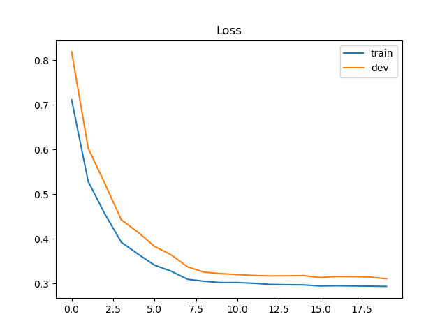
Loss & accuracy
输出最后一次迭代的loss和accuracy。
结果如下:
1 | Training loss: 0.2933570286596322 |
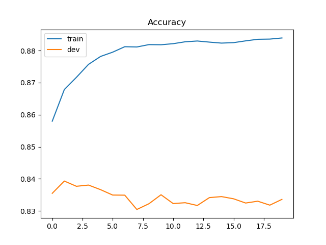
画出loss 和 accuracy的更新过程:
loss:
accuracy:
由于Feature数量较大,将权重影响最大的feature输出看看:
1 | Other Rel <18 spouse of subfamily RP: [7.11323764] |
Code
完整数据集、代码等,欢迎光临小透明GitHub
1 | ################# |
Generative Model
Generative Model 原理部分见 这篇博客
Prepare data
这部分和Logistic regression一样。
只是,因为generative model有closed-form solution,不需要划分development set。
1 | # Prepare data |
Useful functions
1 | # Useful functions |
Training
公式再推导
计算公式:
$$ \begin{equation}\begin{aligned}P\left(C_{1} | x\right)&=\frac{P\left(x | C_{1}\right) P\left(C_{1}\right)}{P\left(x | C_{1}\right) P\left(C_{1}\right)+P\left(x | C_{2}\right) P\left(C_{2}\right)}\\&=\frac{1}{1+\frac{P\left(x | C_{2}\right) P\left(C_{2}\right)}{P\left(x | C_{1}\right) P\left(C_{1}\right)}}\\&=\frac{1}{1+\exp (-z)} =\sigma(z)\qquad(z=\ln \frac{P\left(x | C_{1}\right) P\left(C_{1}\right)}{P\left(x | C_{2}\right) P\left(C_{2}\right)}\end{aligned}\end{equation} $$计算z的过程:
- 首先计算Prior Probability。
- 假设模型是Gaussian的,算出 $\mu_1,\mu_2 ,\Sigma$ 的closed-form solution 。
- 根据 $\mu_1,\mu_2,\Sigma$ 计算出 $w,b$ 。
计算Prior Probability。
程序中用list comprehension处理较简单。
1
2
3
4# compute in-class mean
X_train_0 = np.array([x for x, y in zip(X_train, Y_train) if y == 0])
X_train_1 = np.array([x for x, y in zip(X_train, Y_train) if y == 1])计算 $\mu_1,\mu_2 ,\Sigma$ (Gaussian)
$\mu_0=\frac{1}{C0} \sum_{n=1}^{C0} x^{n} $ (Label=0)
$\mu_1=\frac{1}{C1} \sum_{n=1}^{C1} x^{n} $ (Label=0)
$\Sigma_0=\frac{1}{C0} \sum_{n=1}^{C0}\left(x^{n}-\mu^{}\right)^{T}\left(x^{n}-\mu^{}\right)$ (注意 :这里的 $x^n,\mu$ 都是行向量,注意转置的位置)
$\Sigma_1=\frac{1}{C1} \sum_{n=1}^{C1}\left(x^{n}-\mu^{}\right)^{T}\left(x^{n}-\mu^{}\right)$
$\Sigma=(C0 \times\Sigma_0+C1\times\Sigma_1)/(C0+C1)$ (shared covariance)
1
2
3
4
5
6
7
8
9
10
11
12
13
14
15
16mean_0 = np.mean(X_train_0, axis=0)
mean_1 = np.mean(X_train_1, axis=0)
# compute in-class covariance
cov_0 = np.zeros(shape=(data_dim, data_dim))
cov_1 = np.zeros(shape=(data_dim, data_dim))
for x in X_train_0:
# (D,1)@(1,D) np.matmul(np.transpose([x]), x)
cov_0 += np.matmul(np.transpose([x - mean_0]), [x - mean_0]) / X_train_0.shape[0]
for x in X_train_1:
cov_1 += np.dot(np.transpose([x - mean_1]), [x - mean_1]) / X_train_1.shape[0]
# shared covariance
cov = (cov_0 * X_train_0.shape[0] + cov_1 * X_train_1.shape[0]) / (X_train.shape[0])
计算 $w,b$
在 这篇博客中的第2小节中的公式推导中, $x^n,\mu$ 都是列向量,公式如下:
$$ z=\left(\mu^{1}-\mu^{2}\right)^{T} \Sigma^{-1} x-\frac{1}{2}\left(\mu^{1}\right)^{T} \Sigma^{-1} \mu^{1}+\frac{1}{2}\left(\mu^{2}\right)^{T} \Sigma^{-1} \mu^{2}+\ln \frac{N_{1}}{N_{2}} $$ $w^T=\left(\mu^{1}-\mu^{2}\right)^{T} \Sigma^{-1} \qquad b=-\frac{1}{2}\left(\mu^{1}\right)^{T} \Sigma^{-1} \mu^{1}+\frac{1}{2}\left(\mu^{2}\right)^{T} \Sigma^{-1} \mu^{2}+\ln \frac{N_{1}}{N_{2}}$
但是 ,一般我们在处理的数据集,$x^n,\mu$ 都是行向量。推导过程相同,公式如下:
(主要注意转置和矩阵乘积顺序)
$$ z=x\cdot \Sigma^{-1}\left(\mu^{1}-\mu^{2}\right)^{T} -\frac{1}{2} \mu^{1}\Sigma^{-1}\left(\mu^{1}\right)^{T}+\frac{1}{2}\mu^{2}\Sigma^{-1} \left(\mu^{2}\right)^{T} +\ln \frac{N_{1}}{N_{2}} $$ $w=\Sigma^{-1}\left(\mu^{1}-\mu^{2}\right)^{T} \qquad b=-\frac{1}{2} \mu^{1}\Sigma^{-1}\left(\mu^{1}\right)^{T}+\frac{1}{2}\mu^{2}\Sigma^{-1} \left(\mu^{2}\right)^{T} +\ln \frac{N_{1}}{N_{2}}$
但是,协方差矩阵的逆怎么求呢?
numpy中有直接求逆矩阵的方法(np.linalg.inv),但当该矩阵是nearly singular,是奇异矩阵时,就会报错。
而我们的协方差矩阵(510*510)很大,很难保证他不是奇异矩阵。
于是,有一个 牛逼 强大的数学方法,叫SVD(singular value decomposition, 奇异值分解) 。
原理步骤我……还没有完全搞清楚QAQ(先挖个坑)[1]
利用SVD,可以将任何一个矩阵(即使是奇异矩阵),分界成 $A=u s v^T$ 的形式:其中u,v都是标准正交矩阵,s是对角矩阵。(numpy.linalg.svd方法实现了SVD)
可以利用SVD求矩阵的伪逆
- $A=u s v^T$
- u,v是标准正交矩阵,其逆矩阵等于其转置矩阵
- s是对角矩阵,其”逆矩阵“(注意s矩阵的对角也可能有0元素) 将非0元素取倒数即可。
- $A^{-1}=v s^{-1} u$
计算 $w,b$ 的代码如下:
1 | # compute weights and bias |
Accuracy
accuracy结果:
1 | Training accuracy: 0.8756450899439694 |
也将权重较大的feature输出看看:
1 | age: [-0.51867291] |
Code
具体数据集和代码,欢迎光临小透明GitHub
1 |
|
Reference
- SVD原理,待补充
「机器学习-李宏毅」:HW2-Binary Income Predicting