「Cryptography-MIT6875」: Lecture 3

In this series, I will learn MIT 6.875, Foundations of Cryptography, lectured by Vinod Vaikuntanathan.
Any corrections and advice are welcome. ^ - ^

Topics:

• The Hybrid Argument.
• An application: PRG length extension.
• The notion of pseudorandom functions: Definition, motivation, discussion and comparison with PRGs.
• PRG implies (stateful) secret-key encryption.
• PRFs imply (stateless) secret-key encryption.

Recap

In the previous blog, we defined Computational Indistinguishability that a new definition of security for secret-key encryption, which can overcome Shannon’s impossibility.

Then we brought about Pseudorandom Generator which can encrypt a single message longer than the key. We gave the definition of PRG from the Indistinguishability and proved the secret-key encryption scheme by contradiction.

At the end, we saw a construction of PRG based on subset sum, and answered the question of whether there is a PRG.

Agenda

We already know PRG can encrypt a single message longer than the key.

The last blog left the second question to PRG.

Q2: How to encrypt poly. many messages with a fixed key ?

This is the gist of this blog. We’ll introduce two methods.

1. PRG length extension.
   We can achieve stateful encryption of poly. many messages.

   Theorem:
   If there is a PRG that stretched by one bit, there is one that stretched by poly. many bits.

2. Another new notion: Pseudorandom Functions (PRF)
   We can achieve stateless encryption of poly many messages.

   Theorem(next blog):
   If there is a PRG, then there is a PRF.

More importantly, we’ll introduce a new proof technique, Hybrid Arguments.

PRG

In the last blog, we mentioned that there are three equivalent definitions of PRG.

Def 1 [Indistinguishability]

“No polynomial-time algorithm can distinguish between the output of a PRG on a random seed vs. a truly random string.”

= “as good as” a truly random string for all practical purpose.

Def 2 [Next-bit Unpredictability]

“No polynomial-time algorithm can predict the (i+1)th bit of the output of a PRG given the first i bits, better than chance 1/2.”

Def 3 [ Incompressibility]

“No polynomial-time algorithm can compress the output of the PRG into a shorter string”

Def 1 [Indistinguishability]

We elaborated the first definition of Indistinguishability last blog.

Definition 1 [Indistinguishability]:

A deterministic polynomial-time computable function ${G}:\{0,1\}^n\rightarrow \{0,1\}^m$ is a indistinguishable (or, secure against any statistical test) if:

for every p.p.t. algorithm D (called a distinguisher or a statistical test) if there is a negligible function ${\mu}$ such that:

$$
|\operatorname{Pr}[D({G(U_n)})=1]-\operatorname{Pr}[D({U_m})=1]|={\mu(n)}
$$

Notation: $U_n$(resp. $U_m$) denotes the random uniform distribution on $n$-bit (resp. $m$-bit) strings; $m$ is shorthand for $m(n)$.

So $G$ is a PRG if $D$ cannot distinguish from the output of the $G$ and a truly random string.

Def 2 [Next-bit Unpredictability]

Today I will introduce the second definition of Next-bit Unpredictability.

Definition 2 [Next-bit Unpredictability]:

A deterministic polynomial-time computable function ${G}:\{0,1\}^n\rightarrow \{0,1\}^m$ is a next-bit unpredictable if:

for every p.p.t. algorithm D (called a next-bit predictor) and every $i\in\{0,\dots,m\}$ , if there is a negligible function ${\mu}$ such that:

$$
\operatorname{Pr}[y\leftarrow G(U_n):P(y_1y_2\dots y_{i-1})=y_i]=\frac{1}{2}+\mu(n)
$$

Notation: $y_1,y_2,\dots,y_m$ are the bits of the m-bit string $y$.

So $G$ is a PRG if the probability of $P$ predicting the right $i$th bit of $G$ is substantially half given the first $(i-1)$ bits of $G$.

Ind. = NBU

There are two theorems that state the equivalence of Def 1( Indistinguishability) and Def 2(NBU).

Theorem:

A PRG $G$ is distinguishable if and only if it is next-bit unpredictable.

Theorem:

A PRG $G$ passes all (poly-time) statistical tests if and only if it passes (poly-time) next-bit tests.

---

Next-bit Unpredictability(NBU) is seemingly a much weaker requirement. It only says that the next bit predictors, a particular type of distinguishers which takes a prefix of a string and try yo predict the next bit, cannot succeed.

Yet, surprisingly, Next-bit Unpredictability (NBU) = Indistinguishability (Ind.).

In addition, NBU is much more easier to use.

Ind. → NBU

The first and foremost, the thing we want to prove is that if a PRG $G$ is indistinguishable, then it is next-bit unpredictable, i.e. Ind. → NBU.

Proof:

The main idea of contradiction is that if there exists a p.p.t. predictor $P$, then we can construct a p.p.t distinguisher $D$ from $P$, i.e. NOT NBU → NOT Ind.

So we can

• Suppose for contradiction $G$ is NOT Next-bit Unpredictable, i.e. there is a p.p.t. predictor $P$, a polynomial function $p$ and an $i\in\{1,\dots, m\}$ s.t.

  $$
  \operatorname{Pr}[y\leftarrow G(U_n):P(y_1y_2\dots y_{i-1})=y_i]\ge \frac{1}{2}+1/p(n)
  $$

  Then, I claim that $P$ essentially gives us a distinguisher $D$.

  • The probability of $P$ predicting the right bit is more than half.
  • Consequently, the PRG $G$ is NOT Next-bit Unpredictable.

• Construct a distinguisher $D$ from predictor $P$.
  Consider $D$ which gets an $m$-bit string $y$ and does the following:
  (If $P$ is p.p.t. so is $D$.)

  1. Run $P$ on the $(i-1)$-bit prefix $y_1y_2\dots y_{i-1}$
  2. If $P$ returns the $i$-th bit $y_i’$, then output 1 (=PRG) else output 0 (=Random).
  3. $D(y)=\begin{cases} \text{1(=PRG)},& y_i'=y_i\\ \text{0(=Random)},& \text{otherwise}\end{cases}$
  • The task of $D$ is to guess which world she is in, the pseudorandom world or the truly random world.
  • The task of $P$ is to predict the next-bit given the first $(i-1)$ bits of $y$.
  • By the construction of $D$, the probability of $D$ guessing correctly is equal to the probability of $P$ predicting the right bit regardless the distribution of $y$, i.e.
    • $\operatorname{Pr}[y\leftarrow G(U_n):D(y)=1]=\operatorname{Pr}[y\leftarrow G(U_n):P(y_1y_2\dots y_{i-1})=y_i]$
    • $\operatorname{Pr}[y\leftarrow U_m:D(y)=1]=\operatorname{Pr}[y\leftarrow U_m:P(y_1y_2\dots y_{i-1})=y_i]$

• Therefore, we want to show that $D$ is able to distinguish the PRG $G$ which means $G$ is NOT Indistinguishable, i.e. there is a polynomial $p’$ s.t. $|\operatorname{Pr}[y\leftarrow G(U_n):D(y)=1] - \operatorname{Pr}[y\leftarrow U_m:D(y)=1]|\ge 1/p’(n)$

  • If $y$ is from the pseudorandom world, the probability of $D$ guessing correctly is equal to the probability of $P$ predicting the right bit by the construction of $D$.
    • $|\operatorname{Pr}[y\leftarrow G(U_n):D(y)=1]|$
    • = $\operatorname{Pr}[y\leftarrow G(U_n):P(y_1y_2\dots y_{i-1})=y_i]\ge \frac{1}{2}+1/p(n)$ (by assumption)
  • If $y$ is from the truly world, the probability of $P$ predicting the right bit is 1/2 since $y$ is random.
    • $|\operatorname{Pr}[y\leftarrow U_m:D(y)=1]|$
    • =$\operatorname{Pr}[y\leftarrow U_m:P(y_1y_2\dots y_{i-1})=y_i]=\frac{1}{2}$ ($y$ is random)

• Hence, the advantage of the distinguisher $D$ guessing correctly is
  $|\operatorname{Pr}[y\leftarrow G(U_n):D(y)=1] - \operatorname{Pr}[y\leftarrow U_m:D(y)=1]|\ge 1/p(n)$

• QED.

NBU → Ind.

Furthermore, we want to prove that if a PRG $G$ is next-bit unpredictable, then it is indistinguishable, i.e. NBU → Ind..

Equally, suppose for contradiction that there is a distinguisher $D$, and a polynomial function $p$ s.t.

$$
|\operatorname{Pr}[y\leftarrow G(U_n):D(y)=1] - \operatorname{Pr}[y\leftarrow U_m:D(y)=1]|\ge 1/p(n)
$$

But how to construct a next-bit predictor $P$ out of the distinguisher $D$ ?

It is imperative that we need a new proof technique, HYBRID ARGUMENT.

Using the technique, we can prove it by the following steps:

1. Hybrid Argument
2. From Distinguishing to Predicting

Proof of NBU → Ind.

Step 1: Hybrid Argument

Hybrid Argument is a proof technique used to show that two distributions are computationally indistinguishable. ——wiki

The contradiction is that there is a distinguisher $D$, and a polynomial function $p$ s.t.
$|\operatorname{Pr}[y\leftarrow G(U_n):D(y)=1] - \operatorname{Pr}[y\leftarrow U_m:D(y)=1]|\ge 1/p(n)$

We define the advantage of $D$ guessing correctly is $\varepsilon:=1/p(n)$.

A Puzzle

Before that, let’s discuss a simple puzzle.

Lemma:

Let $p_0,p_1,p_2,\dots,p_m$ be real numbers s.t. $\color{blue}{p_m-p_0\ge \varepsilon}$

Then, there is an index $i$ such that $\color{blue}{p_i-p_{i-1}\ge \varepsilon/m}$.

Proof:

• Write it $p_{m}-p_{0}=\left(p_{m}-p_{m-1}\right)+\left(p_{m-1}-p_{m-2}\right)+\cdots+\left(p_{1}-p_{0}\right) \ge \varepsilon$
• At least one of the $m$ terms has to be at least $\varepsilon/m$ (averaging).

Hybrid Distributions

We define a sequence of hybrid distributions $H_0,H_1,\dots,H_m$, which $H_0:=U_m$ and $H_m:=G(U_n)$.

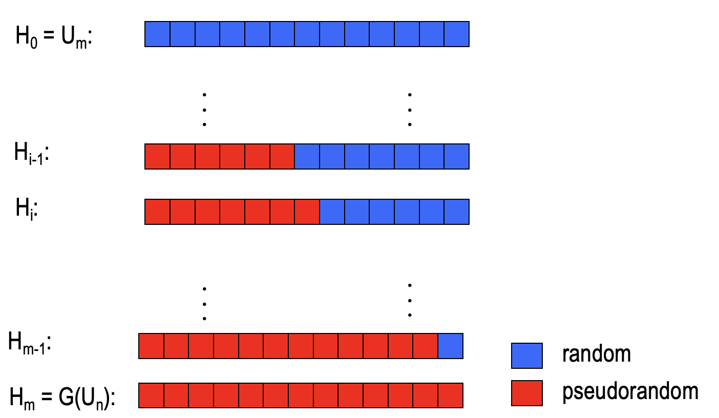
• $H_0$ is the distribution that all bits are random while $H_m$ is the distribution that all bits are pseudorandom.
• Others are the distributions that some bits are random and others are pseudorandom.
• In addition, there is only one different bit between the adjacent hybrid distributions as shown the figure above.

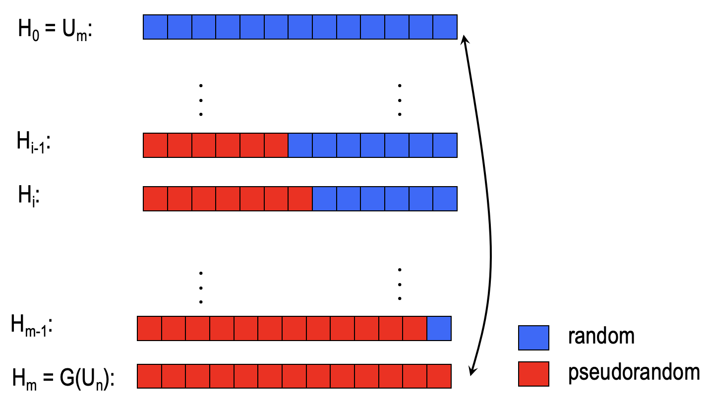
According to the assumption, $D$ distinguishes the $y$ between the pseudorandom world and the truly random world with advantages $\varepsilon$, which means $D$ distinguishes the distribution between $H_m$ and $H_0$ with advantage $\varepsilon$, i.e.

$$
\operatorname{Pr}[D(H_m)=1] - \operatorname{Pr}[D(H_0)=1]\ge \varepsilon
$$

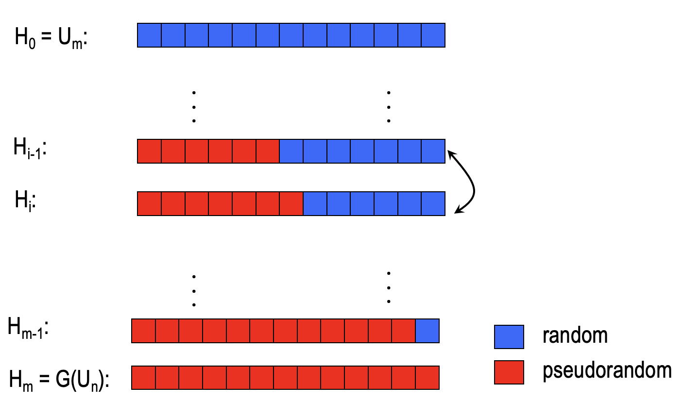
With reference to the puzzle, there exists $i$ such that $D$ distinguishes the distribution between $H_{i}$ and $H_{i-1}$ with advantage $\ge \varepsilon/m$, i.e. $\exists i$ s.t.

$$
\operatorname{Pr}[D(H_i)=1] - \operatorname{Pr}[D(H_{i-1})=1]\ge \varepsilon/m
$$

Random bit v.s. Pseudorandom bit

By the hybrid argument, what information can we get from $D$ distinguishing between $H_{i}$ and $H_{i-1}$with advantage $\ge \varepsilon/m$ ?

Let’s summarize it:

1. Define $p_i = \operatorname{Pr}[D(H_i)=1]$.
   $p_0 = \operatorname{Pr}[D(U_m)=1]$ and $p_m = \operatorname{Pr}[D(G(U_n))=1]$.
2. By the hybrid argument, we have $p_i-p_{i-1}\ge \varepsilon /m$.

The key intuition is $D$ output ‘1’ more often given a pseudorandom $i$-th bit than a random $i$-th bit.

Therefore, $D$ gives us a “signal” as to whether a given bit is the correct $i$-th bit or not.

Right bit v.s. Wrong bit

Let’s dig a bit more.

$H_{i-1}$ is the hybrid distribution the $i$-th bit of which is a random bit $u$.

$H_i$ is the hybrid distribution the $i$-th bit of which is the $i$-th pseudorandom bit $y_i$ generated by $G$.

We define a new hybrid distribution $\overline{H_i}$, the $i$-th bit $\overline{y_i}$ of which is the opposite bit $y_i$ in $H_i$.

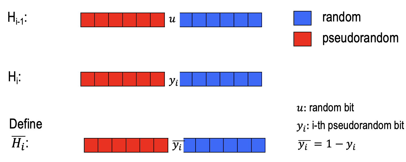
With reference to $p_i=\operatorname{Pr}[D(H_i)=1]$, we define $\overline{p_i}=\operatorname{Pr}[D(\overline{H_i})=1]$.

• We know: $p_i-p_{i-1}\ge \varepsilon/m$.

• Claim: $p_{i-1}=(p_i+\overline{p_i})/2$.
  Proof:

  The following proof is my own deduction since the proof is omitted in the lecture.
  Corrections and advice are welcome.
  • In hybrid distribution $H_{i-1}$, $u$ is a random bit.
    • So, $\operatorname{Pr}[u=0]=0.5$ and $\operatorname{Pr}[u=1]=0.5$.
    • $\operatorname{Pr}[D(H_{i-1})=1]$
    • = $\operatorname{Pr}[D(H_{i-1})=1\wedge u=0]+[D(H_{i-1})=1\wedge u=1]$
    • = $\operatorname{Pr}[D(H_{i-1})=1\mid u=0]\operatorname{Pr}[u=0]+[D(H_{i-1})=1\mid u=1]\operatorname{Pr}[u=1]$
    • =$(\operatorname{Pr}[D(H_{i-1})=1\mid u=0]+[D(H_{i-1})=1\mid u=1])/2$
  • If $u=0$ in $H_{i-1}$, we can use $H_i$ with $y_i=0$ and $\overline{H_{i}}$ with $\overline{y_i}=0$ to express $H_i$.
    • $\operatorname{Pr}[D(H_{i-1})=1\mid u=0]$
    • = $\operatorname{Pr}[D(H_{i-1})=1\wedge y_i=0]+\operatorname{Pr}[D(\overline{H_i})=1\wedge \overline{y_i}=0]$
  • If $u=1$ in $H_{i-1}$, we can use $H_i$ with $y_i=1$ and $\overline{H_{i}}$ with $\overline{y_i}=1$ to express $H_i$.
    • $\operatorname{Pr}[D(H_{i-1})=1\mid u=1]$
    • = $\operatorname{Pr}[D(H_{i-1})=1\wedge y_i=1]+\operatorname{Pr}[D(\overline{H_i})=1\wedge \overline{y_i}=1]$
  • Sum it up.
    • $\operatorname{Pr}[D(H_{i-1})=1]$
    • = $(\operatorname{Pr}[D(H_i)=1\wedge y_i=0] +\operatorname{Pr}[D(H_i)=1\wedge y_i=1] \ + \operatorname{Pr}[D(\overline{H_i})=1\wedge \overline{y_i}=0] +\operatorname{Pr}[D(\overline{H_i})=1\wedge \overline{y_i}=1])/2$
    • = $(\operatorname{Pr}[D(H_i)=1]+\operatorname{Pr}[D(\overline{H_i})=1])/2$
  • QED.

• We illustrate the claim as the following figure.
  $p_{i-1}$ is the midpoint of $p_i$ and $\overline{p_i}$.

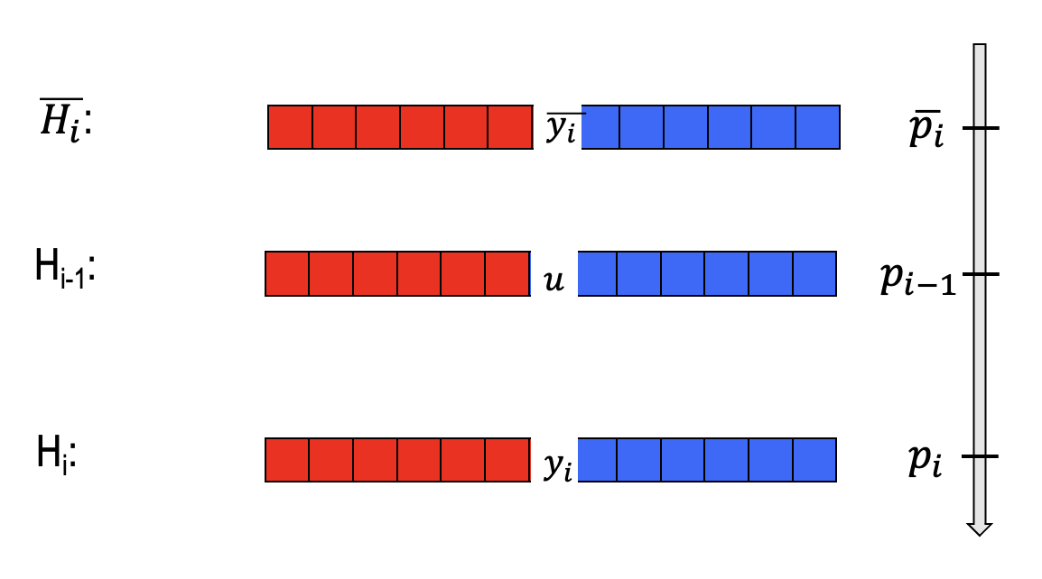
• Corollary: $p_i-\overline{p_i}\ge 2\varepsilon/m$ (w.r.t. the claim)

What can we learn from $p_i-\overline{p_i}\ge 2\varepsilon/m$ ?

The takeaway is that $D$ says ‘1’more often when fed with the ‘right bit’ than the ‘wrong bit’.

Step 2: From Distinguishing to Predicting

By the hybrid argument, we get the takeaway: $p_i-\overline{p_i}\ge 2\varepsilon/m$. ( $p_i=\operatorname{Pr}[D(H_i)=1]$ )

The distinguisher $D$ outputs ‘1’ more often when fed with the ‘right bit’ than the ‘wrong bit’.

The Predictor $P$

The predictor is given the first $i-1$ pseudorandom bits (call it $y_1y_2\dots y_{i-1}$) and needs to guess the $i$-th bit.

The Predictor $P$ works as follows:

$$ P(y_1y_2\dots y_{i-1})=\begin{cases} b,& \text{if }D(y_1y_2\dots y_{i-1}|b| u_{i+1}\dots u_m)=1\\ \overline{b},& \text{otherwise}\end{cases},b\leftarrow\{0,1\} $$

1. Pick a random bit $b$
2. Feed $D$ with input $y_1y_2\dots y_{i-1}|b| u_{i+1}\dots u_m$ ($u$’s are random).
3. If D says ‘1’, output $b$ as the prediction for $y_i$ and if $D$ says ‘0’, output $\overline{b}$ as the prediction for $y_i$.

Analysis of Predictor $P$

• The probability of $P$ predicting the right bit
  $\operatorname{Pr}[x\leftarrow {0,1}^n;y=G(x):P(y_1y_2\dots\ y_{i-1})=y_i]$
• consists of two cases where $D$ outputs 1 and $D$ outputs 0.
  • = $\operatorname{Pr}[D(y_1y_2\dots y_{i-1}b\dots)=1 \wedge b=y_i]+\operatorname{Pr}[D(y_1y_2\dots y_{i-1}b\dots)=0\wedge b\ne y_i]$ ($y_i=b \text{ or } y_i=\overline{b}$)
  • = $\operatorname{Pr}[D(y_1y_2\dots y_{i-1}b\dots)=1 \mid b=y_i]\operatorname{Pr}[b=y_i] \ +\operatorname{Pr}[D(y_1y_2\dots y_{i-1}b\dots)=0\mid b\ne y_i]\operatorname{Pr}[b\ne y_i]$
  • = $\frac{1}{2}(\operatorname{Pr}[D(y_1y_2\dots y_{i-1}y_i\dots)=1]+\operatorname{Pr}[D(y_1y_2\dots y_{i-1}\overline{y_i}\dots)=0)$ (since b is random)
  • = $\frac{1}{2}(\operatorname{Pr}[D(y_1y_2\dots y_{i-1}y_i\dots)=1]+1-\operatorname{Pr}[D(y_1y_2\dots y_{i-1}\overline{y_i}\dots)=1)$
  • = $\frac{1}{2}(1+\varepsilon/m)\ge \frac{1}{2} + 1/p(n)$ (since $m$ is also a polynomial in $n$)
  • QED.

---

SUMMARIZE:

We want to prove that if the $G$ is next-bit predictable, then $G$ is indistinguishable.

1. Hybrid Argument
   1. Suppose the contradiction that there is a $D$ distinguishing from the pseudorandom world and the truly random world with advantage $\varepsilon$.
      $\operatorname{Pr}[y\leftarrow G(U_n):D(y)=1] - \operatorname{Pr}[y\leftarrow U_m:D(y)=1]\ge \varepsilon$
   2. By defining a sequence of hybrid distributions, we know that $D$ outputs ‘1’ more often when fed with a pseudorandom bit than fed a random bit.
      $p_i-p_{i-1}\ge \varepsilon/m \qquad(p_i=\operatorname{Pr}[D(H_i)=1])$
   3. Dig it more. We get the takeaway that $D$ says ‘1’ more often when fed a right bit than a wrong bit.
      $p_i-\overline{p_i}\ge 2\varepsilon/m \qquad(\overline{p_i}=\operatorname{Pr}[D(\overline{H_i})=1])$
2. From distinguishing to predicting
   1. Construct a predictor $P$ from the distinguisher $D$ $P(y_1y_2\dots y_{i-1})=\begin{cases} b,& \text{if }D(y_1y_2\dots y_{i-1}|b| u_{i+1}\dots u_m)=1\\ \overline{b},& \text{otherwise}\end{cases},b\leftarrow\{0,1\}$
   2. Analysis the probability of $P$ predicting the right bit.
      By the hybrid argument, we can deduce $\operatorname{Pr}[x\leftarrow \{0,1\}^n;y=G(x):P(y_1y_2\dots\ y_{i-1})=y_i]\ge1/2+1/p(n)$.
   3. So the probability of $P$ predicting the right bit is more than half.

Proof of PBU = Ind.

We have proven that Next-bit Unpredictability = Indistinguishability.

Actually, Previous-bit Unpredictability(PBU) is equal to Indistinguishability, i.e. PUB = Ind..

I write it down just to exercise.
The proof is similar with the proof of NBU=IND, so you can skip reading it.

Proof:

• Prove PUB → Ind.

  1. Suppose for the contradiction that there is a p.p.t. predictor $P$, a polynomial function $p$ and an $i\in\{1,2,\dots,m\}$ s.t.
     $\operatorname{Pr}[y\leftarrow G(U_n):P(y_{i+1}y_{i+2}\dots y_m)=y_i]\ge 1/2+p(n)$
  2. Construct a distinguisher $D$ from $P$ $D(y)=\begin{cases} \text{1(=PRG)}&, P(y_{i+1}y_{i+2}\dots y_m)=y_i\\ \text{0(=Random)}&, \text{otherwise}\end{cases}$
  3. Analysis the probability of $D$ distinguishing $y$.
     1. If $y$ is from pseudorandom world
        $\operatorname{Pr}[y\leftarrow G(U_n):D(y)=1] \ = \operatorname{Pr}[y\leftarrow G(U_n):P(y_{i+1}y_{i+2}\dots y_m)=y_i]\ge 1/2+p(n)$
     2. If $y$ is from the truly random world
        $|\operatorname{Pr}[y\leftarrow U_m:D(y)=1]| \ =\operatorname{Pr}[y\leftarrow U_m:P(y_{i+1}y_{i+2}\dots y_m)=y_i]= 1/2$
     3. The advantage of $D$ distinguishing $y$ is non-negligible.
        $|\operatorname{Pr}[y\leftarrow G(U_n):D(y)=1] - \operatorname{Pr}[y\leftarrow U_m:D(y)=1]|\ge 1/p(n)$
  4. QED.

• Prove Ind. → PUB

  1. Suppose for the contradiction that there is a p.p.t distinguisher $D$, a polynomial function $p$ s.t.
     $|\operatorname{Pr}[y\leftarrow G(U_n):D(y)=1] - \operatorname{Pr}[y\leftarrow U_m:D(y)=1]|\ge 1/p(n):=\varepsilon$

  2. Hybrid Argument

     1. Define a sequence of hybrid distributions $H_0:=U_m,H_1,\dots,H_m=G(U_n)$
        Define $p_i=\operatorname{Pr}[D(H_i)=1]$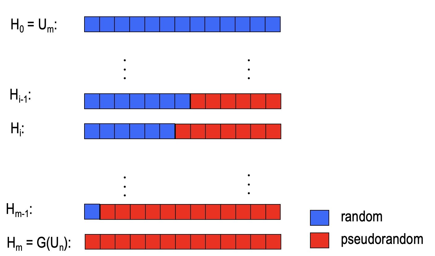

        

     2. We know $p_m-p_0\ge \varepsilon$ from the contradiction.

     3. Define $\overline{p_i}=\operatorname{Pr}[D(\overline{H_i})=1]$ where the $i$-th bit in $\overline{H_i}$ is the opposite bit of the $i$-th bit in $H_i$.

     4. We claim $p_{i-1}=(p_i+\overline{p_i})/2$ . (The proof is same with the above)

        

     5. Get the corollary $p_i-\overline{p_i}\ge 2\varepsilon/m$.
        Takeaway: $D$ output ‘1’ more often when fed with a right bit than a wrong bit.

  3. From distinguishing to predicting

     1. Construct a predictor $P$ from the $D$ $P(y_{i+1}y_{i+2}\dots y_m)\begin{cases} b,& \text{if }D(u_1u_2\dots u_{i-1}|b| y_{i+1}y_{i+2}\dots y_m)=1\\ \overline{b},& \text{otherwise}\end{cases}\\b\leftarrow\{0,1\},u\text{ is random.}$
     2. Analyze the probability of $P$ predicting.
        1. $\operatorname{Pr}[y\leftarrow G(U_n):P(y_{i+1}y_{i+2}\dots y_m)=y_i]$
        2. = $\operatorname{Pr}[D(\dots b y_{i+1}y_{i+2}\dots y_m)=1 \wedge b=y_i]+\operatorname{Pr}[D(\dots b y_{i+1}y_{i+2}\dots y_m)=0\wedge b\ne y_i]$($y_i=b \text{ or } y_i=\overline{b}$)
        3. =$\frac{1}{2}(\operatorname{Pr}[D(\dots y_i y_{i+1}y_{i+2}\dots y_m)=1]+\operatorname{Pr}[D(\dots \overline{y_i} y_{i+1}y_{i+2}\dots y_m)=0)$ (since b is random)
        4. =$\frac{1}{2}(\operatorname{Pr}[D(\dots y_i y_{i+1}y_{i+2}\dots y_m)=1]+1-\operatorname{Pr}[D(\dots \overline{y_i} y_{i+1}y_{i+2}\dots y_m)=1)$
        5. =$\frac{1}{2}(1+\varepsilon/m)\ge \frac{1}{2} + 1/p(n)$
        6. QED.

PRG Length Extension

Let $G:\{0,1\}^n\rightarrow \{0,1\}^{n+1}$ be a pseudorandom generator.

The goal is to used $G$ to generate poly. many pseudorandom bits.

The construction $G’$ consists of poly. many calls of $G$.

• The input of $G’$ is $s_0$ ($n$-bit).
• The output of $G$ is parsed by $b_i||s_i$, which $b_i$ is 1-bit and $s_i$ is $n$-bit.
• The output of $G’$ are poly. many pseudorandom bit.

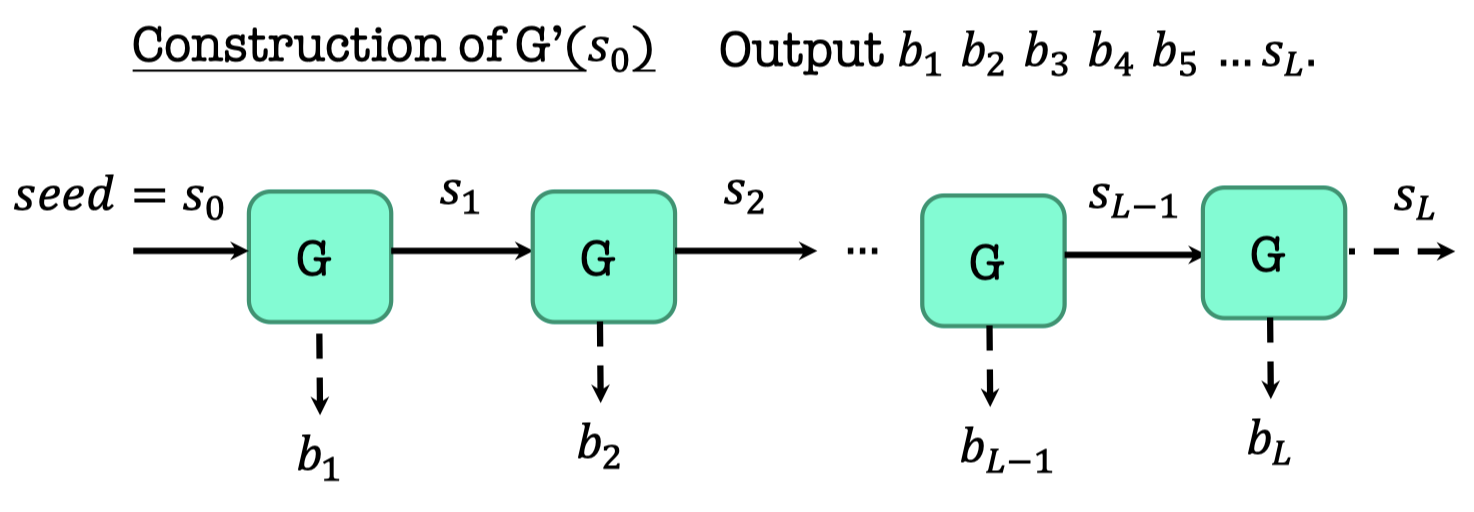
It’s also called a stream cipher by the practitioners.

Security Analysis

Theorem:

If there is a PRG that stretched by one bit, there is one that stretched by poly. many bits.

The following proof is my own deduction since the proof is omitted in the lecture.
Corrections and advice are welcome.

$G:\{0,1\}^n\rightarrow \{0,1\}^{n+1}$ is a PRG that stretched by one bit.

Define $G’(s_0)=b_1b_2\dots b_L$ with the above construction, which is a PRG that stretched by poly. many bits.
$s_0$ is $n$-bit random string and $L$ is a polynomial in $n$.

The thing we want to prove is that if $G:\{0,1\}^n\rightarrow \{0,1\}^{n+1}$ is a secure PRG, then $G':\{0,1\}^n\rightarrow \{0,1\}^{n+L}$ is a secure PRG.

There are many definitions of PRG, but it’s easy to work with Previous-bit Unpredictability here.

Proof:

• Suppose for the contradiction that there is a p.p.t. predictor $P$, who can predict the previous-bit, and a polynomial function $p$ and an $i\in\{1,2,\dots,L\}$ s.t.
  $\operatorname{Pr}[b\leftarrow G’(U_n):P(b_{i+1}b_{i+2}\dots b_L)=b_i] \ge 1/p(n):=\varepsilon$
• Then the predictor $P$ essentially gives us an adversary $A$ against $G$.
  • The task of $A$ is to predict $b_i$ given $s_i$ that $b_i$ is the first bit of $G(s_{i-1})=b_i||s_i$.
  • The construction of $A$
    1. Run $G’$ on the seed $s_i$.
       We can get $b_{i+1},b_{i+2},\dots,b_L$ from the output of $G’(s_i)$.
    2. Feed $P$ with $b_{i+1},b_{i+2},\dots,b_L$.
    3. $A$ returns the output of $P$.
  • Analysis of the adversary $A$ predicting the previous bit.
    • $\operatorname{Pr}[b_i||s_i\leftarrow G(U_n):A(s_i)=b_i]$
    • = $\operatorname{Pr}[(b_{i+1},b_{i+2},\dots,b_L)\leftarrow G’(s_i):P(b_{i+1},b_{i+2},\dots,b_L)=b_i]$
    • = $\operatorname{Pr}[b\leftarrow G’(U_n):P(b_{i+1},b_{i+2},\dots,b_L)=b_i]\ge 1/p(n)$
    • QED.

Stateful Secret-key Encryption

From the PRG length extension, we can encrypt poly. many messages with a fixed key.

The procedure is as follows.

1. Alice and Bob have an agreed key $s_0$ as the initial state of $G’$

   

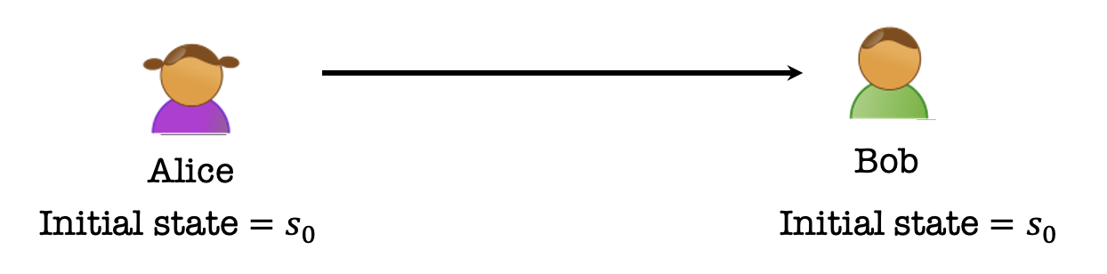
2. Alice wants to encrypt a 1-bit $m$.
   Then Alice and Bob uses $G’(s_0)$ to generate 1 bit $b_1$ as the one-time pad key, and their states convert to $s_1$.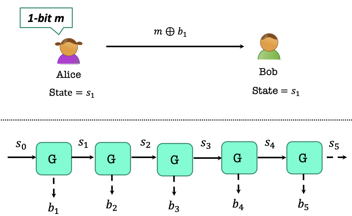

   

3. Alice wants to encrypt a 3-bit $m’$.
   Then Alice and Bob uses $G’(s_1)$ to generate 3 bits $b_2b_3b_4$ as the one-time pad key, and their states convert to $s_4$.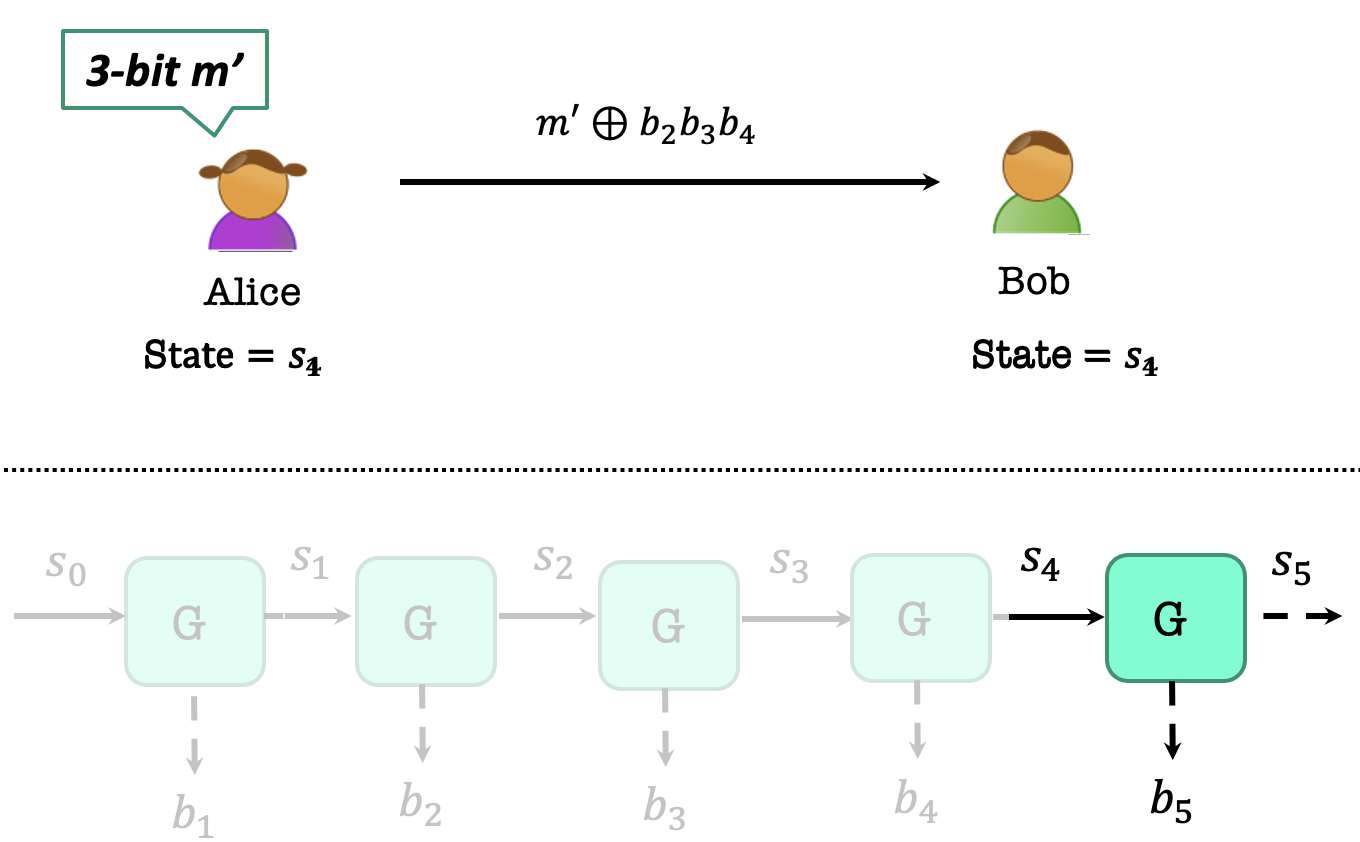

   

4. Now Bob wants to encrypt a 1-bit $m’’$.
   Then Alice and Bob uses $G’(s_4)$ to generate 1 bit $b_5$ as the one-time pad key, and their states convert to $s_5$.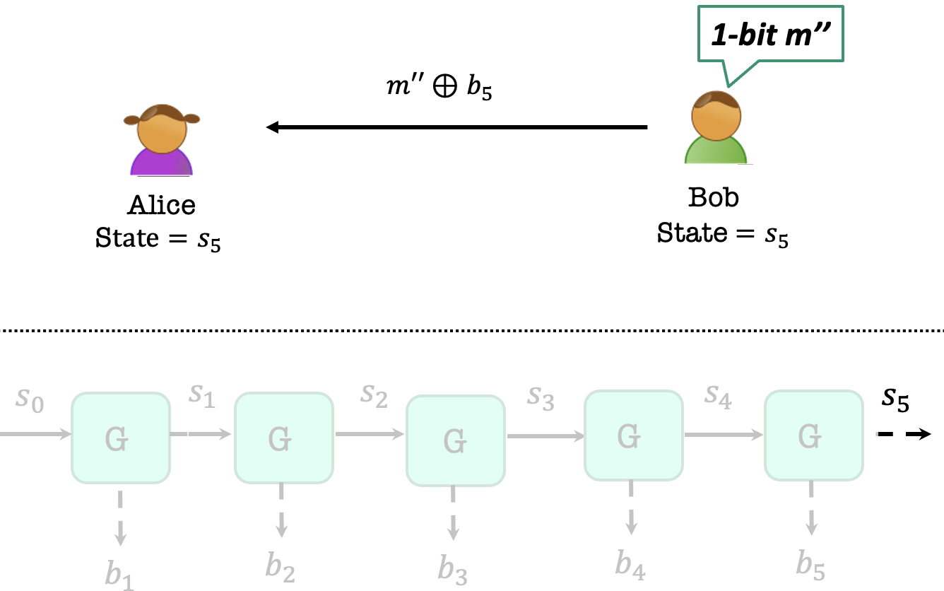

   

---

It’s achievable that Alice and Bob can keep encrypting as many bits as they wish.

However, Alice and Bob have to keep their states in perfect synchrony.

They cannot transmit simultaneously. Otherwise, correctness goes down the drain, so does security.

PRF

It’s stateful encryption using PRG length extension.

How to be stateless ?

There is an idea that Alice and Bob can generate (poly.) many and many bits, such as $n^{100}$ bits.

If Alice want to encrypt 1-bit $m$, she can use a random key $b_x$ indexed by the random number $x$ she picks up and send $(x,m\oplus b_x$) to Bob.

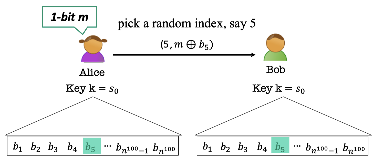
Yet, it dose not work.

Because there is a collision of Alice using the same one-time key with non-negligible probability.
$\operatorname{Pr}[\text{Alice’s first two indices collide}]\ge 1/n^{100}$

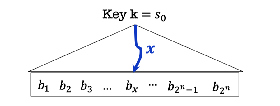
To prevent the collision, there is another idea that Alice and Bob can generate $2^n$ bits and the probability of collision is negligible.
$\operatorname{Pr}[\exists \text{ collision in }t=p(n)\text{ indices}]\le t^2/2^n=neg(n)$

But it brings about another problem that Alice and Bob are not poly-time.

---

Although it dose not work, there is some inspiration.

The goal is never compute the exponentially long string explicitly since it’s not poly-time.

Instead, we want a function $f_k(x)=b_x$, that $b_x$ is the $x$-th bit in the implicitly defined (pseudorandom) string. It is computable in polynomial time $p(|x|)=p(n)$ that $|x|$ is the length of $x$.

And $f_k(x_1),f_k(x_2)\dots$ are computationally indistinguishable from random bits for random $x_1,x_2,\dots$

Hence, there is no need to store the state after each encryption since you can get the encryption key directly by computing the function.

Consequently, it is the stateless encryption of poly. many messages.

The functions are called Pseudorandom Functions.

Definition

Consider these two collections of functions.

Collection of the Pseudorandom Functions:

Consider the collection of pseudorandom functions $\mathcal{F}_l=\{f_k:\{0,1\}^l\rightarrow\{0,1\}^m\}_{k\in\{0,1\}^n}$, each of which maps $l$ bits to $m$ bits.

• indexed by a key $k$.
• $n$ : key length, $l$: input length, $m$: output length.
• Independent parameters, all poly(sec-param)=poly(n).
• #functions in $\mathcal{F}_l\le 2^n$ (single exponential in $n$)

Every (pseudorandom) function is indexed by the key $k$, so if the $k$ is fixed, the function $f_k$ is fixed.

So the number of functions in the pseudorandom world is up to the number of the keys, that is $2^n$.

Collection of ALL Functions:

Consider the collection of ALL functions $ALL_l=\{f:\{\ 0,1\}^l\rightarrow \{0,1\}^m\}$, each of which is maps $l$ bits to $m$ bits.

• #functions in $ALL_l\le 2^{m2^l}$ (doubly exponential in $l$)

For a fixed $m$-bit string in the output space, there are at most $2^l$ possible inputs with different functions. So the number of the functions in the random world is at most $(2^m)^{2^l}=2^{m2^l}$, which is doubly exponential.

---

The #functions in the pseudorandom world is much less than that in the random world.

But the pseudorandom functions should be “indistinguishable” from random.

There are two worlds, the pseudorandom world and the random world.

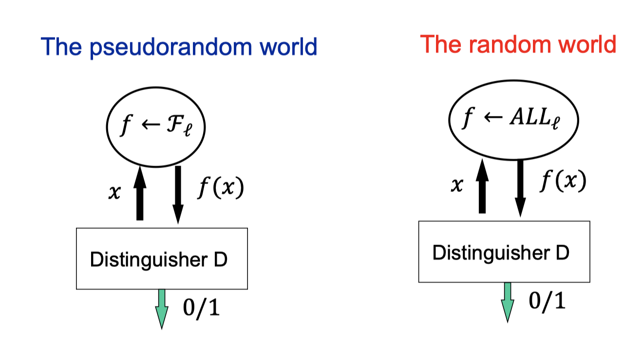
• The pseudorandom world
  1. Sample a function $f$ from $\mathcal{F}_l$.
     The function $f$ is picked one and stays fixed for all. The oracle is instantiated once the $f$ is picked.
  2. The oracle responses $f(x)$ for each query $x$.
     You can think there is a truth table of $f$ in the oracle.
     It responses the same $f(x)$ for the same query $x$ since the function $f$ is fixed.
• The random world
  1. sample a function $f$ from $ALL_l$.
     Likewise, the function $f$ is picked one and stays fixed for all. The oracle is instantiated once the $f$ is picked.
  2. The oracle responses $f(x)$ for each query $x$.
     Likewise, it responses the same $f(x)$ for the same query $x$ since the function $f$ is fixed.
• The Distinguisher $D$ has the power of querying the oracle many poly. times and try to guess which world she is in, the pseudorandom world or the random world.

Definition:

For all p.p.t. $D$, there is a negligible function $\mu$ s.t.

$$
|\operatorname{Pr}[f\leftarrow \mathcal{F}_l:D^f(1^n)=1]-\operatorname{Pr}[f\leftarrow ALL_l:D^f(1^n)=1]|\le \mu(n)
$$

Notation: You can consider the subscript $f$ as an interactive C program, which fed with an input and outputs the result. The distinguisher $D$ actually gets nothing as input except the secure parameter.

Stateless Secret-key Encryption

We can define the stateless secret-key encryption scheme from PRF.

• $Gen(1^n)$: Generate a random $n$-bit key $k$ that defines $f_k:\{0,1\}^l\rightarrow \{0,1\}^m$
  The domain size of $f_k$, $2^l$, had better be super-polynomially large in $n$.
• $Enc(k,m)$: Pick a random $x$ and let the ciphertext $c$ be the pair $(x,y=f_k(x)\oplus m)$.
• $Dec(k,c=(x,y))$: Output $f_k(x)\oplus y$

Correctness

$Dec(k,c)=f_k(x)\oplus y=f_k(x)\oplus f_k(x)\oplus m=m$.

---

Alice and Bob agree with the key $k$, which defines the pseudorandom function $f_k$.

When decrypting, Bob computes the one-time key directly through $f_k(x)$.

They don’t need to store $f_k$( or, the giant truth table), the only thing they need to store is the key $k$.

In the next blog, we’ll introduce the theorem that if there is a PRG, then there is a PRF.