「Cryptography-MIT6875」: Lecture 7

In this series, I will learn MIT 6.875, Foundations of Cryptography, lectured by Vinod Vaikuntanathan.
Any corrections and advice are welcome. ^ - ^

It is indeed possible for $F(x)$ to leak a lot of information about $x$ even if $F$ is one-way.

The hardcore predicate $B(x)$ represent the specific piece of information about $x$ which is hard to compute given $F(x)$.

Topics Covered:

• Definition of one-way functions (OWF)
• Definition of hardcore bit/predicate (HCB)
• One-way permutations → PRG.
  (In fact, one-way functions → PRG, but that’s a much harder theorem.)
• Goldreich-Levin Theorem: every OWF has a HCB.
  (Proof for an important special case.)

One-way Functions

Informally, one-way function is easy to compute and hard to invert.

Definition

In last blog, we introduced briefly the definition of One-way functions.

Take 1 (Not a useful definition):

A function (family) $\{F_n\}_{n\in \mathbb{N}}$ where $F_n:\{0,1\}^n\rightarrow \{0,1\}^{m(n)}$ is one-way if for every p.p.t. adversary $A$, there is a negligible function $\mu$ s.t.

$$ \operatorname{Pr}[x\leftarrow \{0,1\}^n;y=F_n(x):A(1^n,y)=x]\le \mu(n) $$

Consider $F_n(x)=0$ for all $x$.

This is one-way according to the above definition. But it’s impossible to find the inverse even if $A$ has unbounded time.

The probability of guessing the inverse of $0$ is negligible since it is essentially random. But $f(x)=0$ is not one-way function obviously.

Hence, it’s not a useful or meaningful definition.

The right definition should be that it is impossible to find an inverse in p.p.t. rather than the exactly chosen $x$.

One-way Functions Definition:

A function (family) $\{F_n\}_{n\in \mathbb{N}}$ where $F_n:\{0,1\}^n\rightarrow \{0,1\}^{m(n)}$ is one-way if for every p.p.t. adversary $A$, there is a negligible function $\mu$ s.t.

$$ \operatorname{Pr}[x\leftarrow \{0,1\}^n;y=F_n(x):A(1^n,y)=\color{red}{x':y=F_n(x')}]\le \mu(n) $$

I’m not going to ask the adversary to come up with $x$ itself which may be impossible.

Instead, I’m just going to ask the adversary to come up with an $x’$ such that $y$ is equal to $F(x’)$. It’s sort of the pre-image of $y$.

Hence, the adversary can always find an inverse with unbounded time.

But it should be hard with probabilistic polynomial time.

---

Moreover, One-way Permutations are one-to-one one-way functions with $m(n)=n$.

Hardcore Bits

If $F$ is a one-way function, it’s hard to compute a pre-image of $F(x)$ for a randomly chosen $x$.

How about computing partial information about an inverse ?

We saw in last blog that we can tell efficiently if $h$ is quadratic residue.

So for the discrete log function $x=\operatorname{dlog}_g(h)$, computing the least significant bit(LSB) of $x$ is easy.

But MSB turns out to be hard.

Moreover, there are one-way functions for which it is easy to compute the first half of the bits of the inverse.

One-way function family easy to compute the first half of the bits:

There is an obvious fact that if $f(x)$ is one-way, then $f’(r||x)=r||f(x)$ is one-way. ($|r|=|f(x)|$)
It’s hard to compute the pre-image of $f’(r||x)$ because if you can break $f’$ then you can break $f$.
But it’s easy to compute the first half of the bits since they are written in the output.

Nevertheless, there has to be a hardcore set of hard to invert inputs.

Concretely, dose there necessarily exist some bit of $x$ that is hard to compute ?

Particularly, “hard to compute” means “hard to guess with probability non-negligibly better than 1/2” since any bit can be guessed correctly with probability 1/2.

So dose there necessarily exist some bit of $x$ that is hard to guess with probability non-negligibly better than 1/2 ?

Hardcore Bit Def

Hardcore Bit Definition (Take 1):

For any function (family) $F:\{0,1\}^n\rightarrow \{0,1\}^m$ , a bit $i=i(n)$ is hardcore if for every p.p.t. adversary $A$, there is a negligible function $\mu$ s.t.

$$ \operatorname{Pr}[x\leftarrow \{0,1\}^n;y=F(x):A(y)=x_i]\le 1/2 +\mu(n) $$

The definition says that it is hard to guess the $i$-th bit of the inverse given the $y$.

I mentioned above that there are one-way functions for which it is easy to compute the first half of the bits of the inverse.

Moreover, there are functions that are one-way, yet every bit is somewhat easy to predict with probability $\frac{1}{2}+1/n$.

This is actually an (hard) exercise in the lecture.

Sadly, I haven’t figured out the construction that every bit is easy to compute w.p. $\frac{1}{2}+1/n$.
Hope to change the ideas with you.

Although the entire inverse of $f(x)$ is hard to compute, it is indeed possible for $f(x)$ to leak a lot of information about $x$ even if $f$ is one-way.

Hardcore Predicate Def

So, we generalize the notion of a hardcore “bit”.

We define hardcore predicate to identify a specific piece of information about $x$ that is “hidden” by $f(x)$.

Informally, a hardcore predicate of a one-way function $f(x)$ is hard to compute given $f(x)$.

Hardcore Predicate Definition:

For any function (family) $F:\{0,1\}^n\rightarrow \{0,1\}^m$ , a function $B:\{0,1\}^n\rightarrow \{0,1\}$ is a hardcore predicate if for every p.p.t. adversary $A$, there is a negligible function $\mu$ s.t.

$$ \operatorname{Pr}[x\leftarrow \{0,1\}^n;y=F(x):A(y)=B(x)]\le 1/2 +\mu(n) $$

The definition says that a hardcore predicate $B(x)$ of a one-way function $f(x)$ is hard to compute with probability non-negligibly better than $1/2$ given $f(x)$ since the predicate $B(x)$ is a boolean function that can be computed with probability $1/2$.

Besides, this is perfectly consistent with the fact that the entire inverse is actually hard to compute. Otherwise, you can compute $B(x)$.

---

Henceforth, for us, a hardcore bit will mean a hardcore predicate.

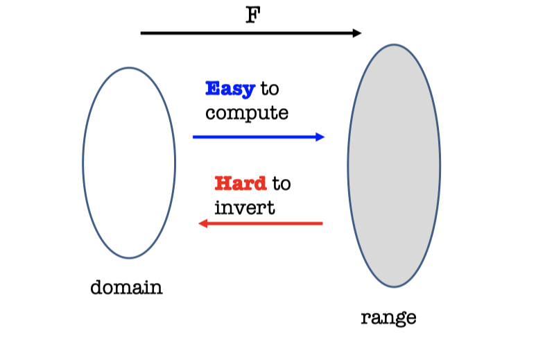
We can represent the definition by the following picture.

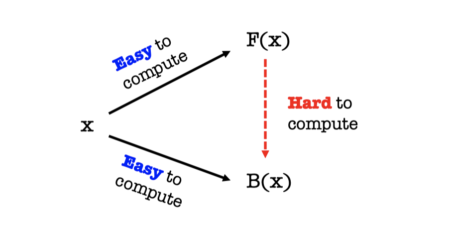
It’s easy to compute the one-way function $F(x)$ given $x$.

It’s easy to compute the hardcore predicate $B(x)$ of $F(x)$ given $x$.

But it’s hard to compute $B(x)$ given $F(x)$.

We know that it is indeed possible for $F(x)$ to leak a lot of information about $x$ even if $F$ is one-way.

Hence, the hardcore predicate $B(x)$ represent the specific piece of information about $x$ which is hard to compute given $F(x)$.

One-way Permutations → PRG

In this section, we show that One-way Permutations imply PRG.

The construction is as follows:

PRG Construction from OWP:

Let $F$ be a one-way permutation, and $B$ an associated hardcore predicate for $F$.

Then, define $G(x)=F(x)||B(x)$.

Note: $G$ stretches by one bit. We can turn this into a $G’$ that stretches to any poly. number of bits from PRG Length Extension.

Theorem:

$G$ is a PRG assuming $F$ is a one-way permutation.

Proof (using NBU):

The thing we want to prove is that if $F$ is a one-way permutation and $B$ is the hardcore predicate for $F$, then $G(x)=F(x)||B(x)$ is a PRG.

We prove it using next-bit unpredictability.

• Assume for contradiction that $G$ is not a PRG.

  Therefore, there is a next-bit predictor $D$, and index $i$, and a polynomial function $p$ such that

  $\operatorname{Pr}[x\leftarrow \{0,1\}^n;y=G(x):D(y_1\dots y_{i-1})=y_i]\ge \frac{1}{2}+1/p(n)$

• If we want to get the contradiction to $B(x)$, the index $i$ has to be $n+1$.
  (Because the $G(x)=F(x)||B(x)$ where $F(x)$ is $n$-bit and $B(x)$ is $1$-bit.)

  $\operatorname{Pr}[x\leftarrow \{0,1\}^n;y=G(x):D(y_1\dots y_{n})=y_{n+1}]\ge \frac{1}{2}+1/p(n)$

• Then we can construct a hardcore bit (predicate) predictor from $D$.
  In fact, $D$ is a hardcore predictor.

  $\operatorname{Pr}[x\leftarrow \{0,1\}^n;y=G(x):D(F(x))=B(x)]\ge \frac{1}{2}+1/p(n)$

• QED.

Proof (using Indistinguishability):

We can also prove it using indistinguishability.

• Assume for contradiction that $G$ is not a PRG.
  Therefore, there is a p.p.t. distinguisher $D$, and a polynomial function $p$ such that

  $$ \begin{aligned}\operatorname{Pr}[x\leftarrow \{0,1\}^n;y=G(x):D(y)=1] &- \\ \operatorname{Pr}[y\leftarrow \{0,1\}^{n+1}:D(y)] &\ge 1/p(n)\end{aligned} $$

• We construct a hardcore predictor $A$ and show:

  $$ \begin{aligned}\operatorname{Pr}[x\leftarrow \{0,1\}^n:A(F(x))=B(x)]\ge \frac{1}{2}+1/p'(n)\end{aligned} $$

• What information can we learn from the distinguisher $D$ ?

  • Rewrite $y$ in the first term by definition.

    $$ \begin{aligned}\operatorname{Pr}[x\leftarrow \{0,1\}^n;y=\color{blue}{F(x)||B(x)}:D(y)=1] &- \\\operatorname{Pr}[y\leftarrow \{0,1\}^{n+1}:D(y)=1]&\ge 1/p(n)\end{aligned} $$

  • Rewrite the second term by a syntactic change.

    $$ \begin{aligned}\operatorname{Pr}[x\leftarrow \{0,1\}^n;y=F(x)||B(x):D(y)=1]&-\\ \operatorname{Pr}[{\color{blue}{y_0\leftarrow \{0,1\}^{n},y_1\leftarrow \{0,1\}},y=y_0||y_1}:D(y)=1] &\ge 1/p(n)\end{aligned} $$

  • Rewire the second term since $F$ is one-way permutation.

    $$ \begin{aligned}\operatorname{Pr}[x\leftarrow \{0,1\}^n;y=F(x)||B(x):D(y)=1]&-\\ \operatorname{Pr}[{\color{blue}{x\leftarrow \{0,1\}^{n},y_1\leftarrow \{0,1\},y=F(x)||y_1}}:D(y)=1] &\ge 1/p(n)\end{aligned} $$ ​

  • Rewrite the second term since $\operatorname{Pr}[y_1=0]=\operatorname{Pr}[y_1=0]=1/2$.

    $$ \begin{aligned}\operatorname{Pr}[x\leftarrow \{0,1\}^n;y=F(x)||B(x):D(y)=1] &-\\ \frac{\operatorname{Pr}[{x\leftarrow \{0,1\}^{n},\color{blue}{y=F(x)||0}}:D(y)=1]+\operatorname{Pr}[{x\leftarrow \{0,1\}^{n},\color{blue}{y=F(x)||1}}:D(y)=1]}{2} &\ge 1/p(n)\end{aligned} $$

  • Rewrite the second term using $B(x)$.

    $$ \begin{aligned}\operatorname{Pr}[x\leftarrow \{0,1\}^n;y=F(x)||B(x):D(y)=1] &-\\ \frac{\operatorname{Pr}[{x\leftarrow \{0,1\}^{n},\color{blue}{y=F(x)||B(x)}}:D(y)=1]+\operatorname{Pr}[{x\leftarrow \{0,1\}^{n},\color{blue}{y=F(x)||\overline{B(x)}}}:D(y)=1]}{2} &\ge 1/p(n)\end{aligned} $$

  • Putting thins together.

    $$ \begin{aligned}\frac{1}{2}(\operatorname{Pr}[{x\leftarrow \{0,1\}^{n},\color{blue}{y=F(x)||B(x)}}:D(y)=1] &- \\ \operatorname{Pr}[{x\leftarrow \{0,1\}^{n},\color{blue}{y=F(x)||\overline{B(x)}}}:D(y)=1]) &\ge 1/p(n)\end{aligned} $$

Although the mathematical transformations seem complex, the main idea is to turn what we know to what we want.

We want to know some information about $B(x)$.

• The takeaway is that $D$ says 1 more often when fed with the “right bit” than the “wrong bit”.

It’s a familiar statement.

In [Lecture 3] , we construct a predictor from a distinguisher to prove the next-bit unpredictability → the indistinguishability.

In that proof, we got the takeaway from hybrid argument, that the distinguisher $D$ says 1 more often when fed with the “right bit” than the “wrong bit”.

• Construct a hardcore bit predictor $A$ from the distinguisher $D$ using the takeaway.

  • The task of $A$ is get as input $z=F(x)$ and try to guess the hardcore predicate.

  • The predictor works as follows:

    $$ \begin{aligned}A(F(x))=\begin{cases} b,& \text{if }D(F(x)||b)=1\\ \overline{b},& \text{otherwise}\end{cases},b\leftarrow\{0,1\} \end{aligned} $$
    1. Pick a random bit $b$.
    2. Feed $D$ with input $z||b$
    3. If $D$ says “1”, output $b$ as the prediction for the hardcore bit and if $D$ says “0”, output $\overline{b}$.

• Analysis of the predictor $A$.

  • $\operatorname{Pr}[x\leftarrow {0,1}^n:A(F(x))=B(x)]$
  • $A$ output $b=B(x)$ or $\overline{b}=B(x)$. $\begin{aligned} =\operatorname{Pr}[x\leftarrow\{0,1\}^n:D(F(x)||b)=1 \color{blue}{\wedge b=B(x)}] + \\ \operatorname{Pr}[x\leftarrow\{0,1\}^n:D(F(x)||b)=0 \color{blue}{\wedge b\ne B(x)}]& \\\end{aligned}$ $\begin{aligned}=\operatorname{Pr}[x\leftarrow\{0,1\}^n:D(F(x)||b)=1 \mid b=B(x)]\operatorname{Pr}[b=B(x)]& + \\ \operatorname{Pr}[x\leftarrow\{0,1\}^n:D(F(x)||b)=0 \mid b\ne B(x)]\operatorname{Pr}[b\ne B(x)]& \end{aligned}$
  • Since $b$ is random.
    $\begin{aligned}=\color{blue}{\frac{1}{2}}(\operatorname{Pr}[x\leftarrow{0,1}^n:D(F(x)||b)=1 \mid b=B(x)]& + \ \operatorname{Pr}[x\leftarrow{0,1}^n:D(F(x)||b)=0 \mid b\ne B(x)]&) \end{aligned}$
  • Put the prior condition in it.$\begin{aligned}=\frac{1}{2}(\operatorname{Pr}[x\leftarrow\{0,1\}^n:D(F(x)||\color{blue}{B(x)})=1]& + \\ \operatorname{Pr}[x\leftarrow\{0,1\}^n:D(F(x)||\color{blue}{\overline{B(x)}})=0 ) \end{aligned}$ $\begin{aligned}=\frac{1}{2}(\operatorname{Pr}[x\leftarrow\{0,1\}^n:D(F(x)||\color{blue}{B(x)})=1]& + \\ 1-\operatorname{Pr}[x\leftarrow\{0,1\}^n:D(F(x)||\color{blue}{\overline{B(x)}})=1 ) \end{aligned}$
  • From the takeaway, we can get
    $=\frac{1}{2}(1+(*))\ge \frac{1}{2} + 1/p(n)$
  • So the $A$ can predict the hardcore bit (predicate) with probability non-negligible better than $1/2$.

Goldreich-Levin Theorem: every OWF has a HCB.

A Universal Hardcore Predicate for all OWF

We have defined the hardcore predicate $B(x)$ for the particular one-way function $F(x)$.

Let’s shoot for a universal hardcore predicate for every one-way function, i.e., a single predicate $B$ where it is hard to guess $B(x)$ given $F(x)$.

Is this possible ?

Turns out the answer is “no”.

Pick a favorite amazing $B$. We can construct a one-way function $F$ which $B$ is not hardcore.

There is a contradiction example.

Claim 1: If $f(x)$ is a one-way function, then $f’(x)=f(x)||B(x)$ is one-way as well.
Claim 2:
But $B(x)$ is NOT a hardcore predicate for $f’(x)$.

For claim 1, if you can compute the inverse of $f’(x)$, then you can compute the inverse of $f(x)$.
For claim 2, $B(x)$ is actually written in $f’(x)$.
So $f’(x)$ is one-way and dose not leak much information.

Goldreich-Levin(GL) Theorem

But Goldreich-Levin(GL) Theorem changes the statement to a random hardcore and tells us every one-way function has a hardcore predicate/bit.

Goldreich-Levin(GL) Theorem:

Let $\{B_r:\{0,1\}^n\rightarrow \{0,1\}\}$ where

$$ B_r(x)=\langle r, x \rangle =\sum_{i=1}^n r_ix_i \mod 2 $$

be a collection of predicates (one for each $r$).

Then a random $B_r$ is hardcore for every one-way function $F$.

That is, for every one-way function $F$, every p.p.t. $A$, there is a negligible function $\mu$ s.t.

$$ \operatorname{Pr}[x\leftarrow \{0,1\}^n;r\leftarrow \{0,1\}^n:A(F(x),r)=B_r(x)]\le\frac{1}{2} +\mu(n) $$

It defines a collection of predicates ${B_r:{0,1}^n\rightarrow {0,1}}$ indexed by $r$, a $n$-bit vector. So the evaluation of $B_r(x)$ is essentially an inner product of $r$ and $x$ (mod 2).

The definition says that a random $B_r$ is hardcore for every one-way funciton $F$.

So it picks a random $x$ and a random $r$.

For every p.p.t. adversary $A$, it is hard to compute $B_r(x)$ given $F(x)$ and $r$.

Alternative Interpretations to GL Theorem

There are some alternative interpretations to GL Theorem.

Alternative Interpretation 1:

For every one-way function $F$, there is a related one-way function $F’(x,r)=(F(x),r)$ which has a deterministic hardcore predicate.

---

For every one-way function $F$, you can change it to a related one-way function $F’(x,r)=(F(x),r)$. Although $F’$ leak the second half of bits, $F’$ is one-way.

Then $F’$has a deterministic hardcore predicate $B(x,r)=\langle x,r \rangle\pmod 2$.

$B(x,r)$ is a fixed function, which performs an inner-product mod 2 between the first half and the second half of the inputs.

Hence, in this interpretation, GL Theorem says that $B$ is not a hardcore bit for every OWF, but it’s a hardcore bit for the related function, which we created it from the OWF.

Moreover, if $F(x)$ is one-way permutation, then $F’(x,r)=(F(x),r)$ is one-way permutation.

And we can get a PRG from $F’(x,r)$. Then $G(x,r)=F(x)||r||\langle x,r\rangle$ where the last bit is the hardcore bit.

Alternative Interpretation 2:

For every one-way function $F$, there exists (non-uniformly) a (possibly different) hardcore predicate $\langle r_F,x\rangle$.

To be honest, I do not comprehend the advanced statement.

The professor left a cool open problem: remove the non-uniformity.

Proof of GL Theorem

Assume for contradiction there is a predictor $P$ and a polynomial $p$ s.t.

$\operatorname{Pr}[x\leftarrow {0,1}^n;r\leftarrow {0,1}^n:P(F(x),r)=\langle r,x\rangle]\ge\frac{1}{2} +p(n)$

We need to show an inverter $A$ for $F$ and a polynomial $p’$ such that

$\operatorname{Pr}[x\leftarrow {0,1}^n:A(F(x))=x’:F(x’)=F(x)]\ge 1/p’(n)$

But it is too hard to prove this contradiction.

Let’s make our lives easier.

A Perfect Predicator

For simplicity, we assume a perfect predicator.

Assume a perfect predictor:

• Assume a perfect predictor $P$, which can completely predicte the HCB correctly, s.t.

  $\operatorname{Pr}[x\leftarrow \{0,1\}^n;r\leftarrow \{0,1\}^n:P(F(x),r)=\langle r,x\rangle]=1$

• Now we can construct an inverter $A$ for $F$.

  The inverter $A$ works as follows:

  On input $y=F(x)$, $A$ runs the predictor $P$ $n$ times on input $(y, e_1),(y,e_2),\dots,$and $(y,e_n)$ where $e_1=100..0,e_2=010..0,\dots$ are the unit vectors.

• Since $A$ is perfect, it returns $\langle e_i,x\rangle=x_i$, the $i$-th bit of $x$ on the $i$-th invocation.

A Pretty Good Predictor

Then we assume less.

Assume a pretty good predictor:

• Assume a pretty good predictor $P$, s.t. $\operatorname{Pr}[x\leftarrow \{0,1\}^n;r\leftarrow \{0,1\}^n:P(F(x),r)=\langle r,x\rangle]\ge \frac{3}{4} + 1/p(n)$
• What can we learn from the predictor ?

Claim:
For at least a $1/2p(n)$ fraction of the $x$,
$\operatorname{Pr}[r\leftarrow {0,1}^n:P(F(x),r)=\langle r,x\rangle]\ge \frac{3}{4} + 1/2p(n)$

How to derive the claim by averaging argument ?

When I wrote this blog, I contemplated it for a long long time.
I figured it out with the help of Wengjie Li. Thanks!
I read the details about the proof of GL Theorem in some textbooks.
Some proved the lower bound of fraction $1/2p(n)$, but how about the lower bound of probability, $\frac{3}{4}+1/2p(n)$?
In fact, they are related.

Before that, let’s introduce averaging argument.

In computational complexity theory and cryptography, averaging argument is a standard argument for proving theorems. It usually allows us to convert probabilistic polynomial-time algorithms into non-uniform polynomial-size circuits.
——Wiki

Averaging Argument:

Let $f$ be some function. The averaging argument is the following claim:

If we have a circuit $C$ such that $C(x,y)=f(x)$ with probability at least $\rho$ where $x$ is chosen at random and $y$ is chosen independently from some distribution $Y$ over $\{0,1\}^m$ (which might not even be effciently sampleable),

then there exists a single string $y_0\in \{0,1\}^m$ such that $\operatorname{Pr}_x[C(x,y_0)=f(x)]\ge \rho$.

---

Indeed, for every $y$ define $p_y$ to be $\operatorname{Pr}_x[C(x,y)=f(x)]$, then

$$ \operatorname{Pr}_{x,y}[C(x,y)=f(x)]=\mathbb{E}_y[p_y] $$

and then this reduces to the claim that for every random variable $Z$, if $\mathbb{E}[Z]\ge \rho$ then $\operatorname{Pr}[Z\ge \rho]>0$ (this holds since $\mathbb{E}[Z]$ is the weighted average of Z and clearly if the average of some values is at least $\rho$ then one of the values must be at least $\rho$.)

The claim tells us if $\operatorname{Pr}_{x,y}[C(x,y)=f(x)]\ge \rho$, then there exist some $y_0$ such that $\operatorname{Pr}_x[C(x,y_0)=f(x)]\ge \rho$ as well.

So we can single out these $y_0$ using averaging argument.

Actually, I think the equation, $\operatorname{Pr}_{x,y}[C(x,y)=f(x)]=\mathbb{E}_y[p_y]$, is the manifestation of averaging.

The following analysis is mostly my own deduction and comprehension since the proof is omitted in the lecture.
Corrections and advice are welcome.

Some analysis to $\operatorname{Pr}_{x,y}[C(x,y)=f(x)]=\mathbb{E}_y[p_y]$:

• By definition of $p_y$
  • $y$ is a variable and $p_y$ is a variable.
  • By definition, $p_y$ is up to $y$.
  • So the distribution of $p_y$ is equal to the distribution of $y$.
• Expand the left term.
  $\operatorname{Pr}_{x,y}[C(x,y)=f(x)]=\sum _i \operatorname{Pr}_x[C(x,y_i)=f(x)]\operatorname{Pr}[y=y_i]$
• The right term is the expected value of variable $p_y$.
  • $\mathbb{E}_y[p_y] = \sum_i p_{y_i} \cdot \operatorname{Pr}[p_y=p_{y_i}]$
  • Because the distribution of $p_y$ is equal to the distribution of $y$.
    $\operatorname{Pr}[p_y=p_{y_0}]=\operatorname{Pr}[y={y_0}]$
  • So, $\mathbb{E}_y[p_y] = \sum_i p_{y_i} \cdot \operatorname{Pr}[y=y_i]$
  • = the left term.

---

Now back to the claim.

The following is mostly my own deduction and comprehension since the proof is omitted in the lecture.
Corrections and advice are welcome.

Proof of the Claim :

What can we learn from the claim?

• What do we know from the predictor ?
  • We know $\operatorname{Pr}_{x,r}[P(F(x),r)=\langle r,x\rangle]\ge \frac{3}{4} + 1/p(n)$.
  • For every $x$, define $p_x=\operatorname{Pr}_r[P(F(x),r)=\langle r,x\rangle]$.
  • By averaging argument,
    1. We know there exists some $x$ such that $p_x\ge \frac{3}{4} + 1/p(n)$.
    2. We know $\operatorname{Pr}_{x,r}[P(F(x),r)=\langle r,x\rangle]=\mathbb{E}[p_x]$ by averaging argument.
    3. So we know the lower bound of $\mathbb{E}[p_x]$ (expected value of $p_x$) is $\frac{3}{4} + 1/p(n)$.
• What do we really want ?
  • We want to single out these $x$ such that $p_x$ is non-negligibly better than $\frac{3}{4}$ in (probabilistic) polynomial time.
  • So we want a set of $x$, which the fraction is polynomial , for every $x$ in the set, the $p_x$ is non-negligibly better than $\frac{3}{4}$.
• We show the fraction and the (lower bound of ) probability are related.
• Notation
  • $\epsilon$ define the lower bound of $\mathbb{E}[p_x]$, i.e. $\epsilon =\frac{3}{4} + 1/p(n)$.
  • Define a good set of $x$ as $S$ and $s$ denotes the poly. fraction of the $x$. ($|S|=s\cdot 2^n$). $S=\{x\mid p_x \ge \varepsilon' \}$
    where $\varepsilon’$ denotes the lower bound of $p_x$ for every $x\in S$, non-negligibly better than $\frac{3}{4}$.
• Rewrite $\mathbb{E}[p_x]$ using $s$ and $\varepsilon$.
  • $p_x= \begin{cases} \varepsilon' \le p_x\le 1,& x\in S \\ 0\le p_x \le \varepsilon',& x\notin S \end{cases}$
  • Similarly, $p_x$ is up to $x$.
    Hence, the distribution of $p_x$ is equal to the distribution of $x$, i.e.$\operatorname{Pr}[p_x]=\operatorname{Pr}[x]$
  • $\mathbb{E}[p_x] = \sum p_x \cdot \operatorname{Pr}[p_x]=\sum p_x \cdot \operatorname{Pr}[x]$
    • $=\sum p_x \cdot \operatorname{Pr}[x\in S] + \sum p_x \cdot \operatorname{Pr}[x\notin S]$
    • $=\sum p_x \cdot s + \sum p_x \cdot (1-s)$
  • We do not know the actual $p_x$ but we know the boundary of $p_x$.
• Calculate the boundary of $\mathbb{E}[p_x]$ using $s$ and $\varepsilon$.
  • $\mathbb{E}[p_x] =\sum p_x \cdot s + \sum p_x \cdot (1-s)$
  • The lower bound is $\varepsilon’ \cdot s + 0\cdot (1-s)=\varepsilon’ \cdot s$ (useless)
  • The upper bound is $1\cdot s + \varepsilon’ \cdot (1-s)=s+\varepsilon’ (1-s)$ (useful)
  This upper bound should be greater than the known lower bound $\epsilon$.
• We get the relation of $s$ and $\varepsilon’$.
  • $\epsilon \le s+\varepsilon’ (1-s)$
  • $\frac{\epsilon-s}{1-s}\le \varepsilon’$ (since $s<1$)
• Take $\epsilon$ with $\frac{3}{4} + 1/p(n)$.
  • We want the fraction $s$ to be polynomial.
  • Suppose the fraction $s=1/2p(n)$.
    We can get $\varepsilon’ \ge \epsilon -s = \frac{3}{4} +1/2p(n)$. (since $1-s$ is very small).
  • We can also suppose the fraction $s=1/3p(n)$ and so on.
  • The point I want to elucidate here is the fraction $s$ and the lower bound of $p_x$ for every $x\in S$ can both be polynomial if the advantage of predicting is non-negligible.
• Hence, the takeaway is if the probability of predicting is non-negligibly better than $3/4$, then we can single out these “good $x$ ”in (probabilistic) polynomial time.
• Similarly, if the probability of predicting is non-negligibly better than $1/2$ (the predictor in general case), we can also single out these “good $x$ ” in (probabilistic) polynomial time.

---

We get the takeaway that if the probability of predicting is non-negligibly better than $3/4$, then we can single out these “good $x$ ” in (probabilistic) polynomial time.

Invert the i-th bit:

• Now we can compute the $i$-th bit of $x$ with the probability better than $1/2$.
  The key idea is linearity.

  1. Pick a random $r$
  2. Ask $P$ to tell us $\langle r,x\rangle$ and $\langle r+e_i,x \rangle$.
  3. Subtract the two answers to get $\langle e_i,x\rangle =x_i$

• Proof of invert $i$-th bit:

  • $\operatorname{Pr}[\text{we compute }x_i \text{ correctly}]$

  • $\ge \operatorname{Pr}[P \text{ predicts }\langle r,x \rangle \text{ and }\langle r+e_i,x \rangle \text{ correctly}]$

  • $=1-\operatorname{Pr}[P \text{ predicts }\langle r,x \rangle \text{ or }\langle r+e_i,x \rangle \text{ wrong}]$

  • $\ge1-\operatorname{Pr}[P \text{ predicts }\langle r,x \rangle \text{ wrong}]\text{ + } \operatorname{Pr}[P \text{ predicts }\langle r+e_i,x \rangle \text{ wrong}]$
    (by union bound)

  • $\ge 1 - 2\cdot (\frac{1}{4} -\frac{1}{2p(n)})=\frac{1}{2}+1/p(n)$

    I think it takes the fraction as $1/2p(n)$ just to make the advantage equal to $1/p(n)$. It’s beautiful.

Invert the entire x:

• Construct the Inverter $A$
  • Repeat for each bit $i\in{1,2,\dots, n}$:
    • Repeat $p(n) \cdot p(n)$ times:
      (one $p(n)$ is for singling out, and another is for computing correctly)
      1. Pick a random $r$
      2. Ask $P$ to tell us $\langle r,x\rangle$ and $\langle r+e_i,x \rangle$.
      3. Subtract the two answers to get $\langle e_i,x\rangle =x_i$
    • Compute the majority of all such guesses and set the bit as $x_i$.
  • Output the concatenation of all $x_i$ as $x$.
• Analysis of $A$ is ommited.
  Hint: Chernoff + Union Bound.

A General Predictor

Let’s proceed to a general predictor, which is in the foremost contradiction.

Assume a general good predictor:

Assume there is a predictor $P$ and a polynomial $p$ s.t.

$\operatorname{Pr}[x\leftarrow \{0,1\}^n;r\leftarrow \{0,1\}^n:P(F(x),r)=\langle r,x\rangle]\ge\frac{1}{2} +p(n)$

Likewise, there is a similar claim.

Claim:

For at least a $1/2p(n)$ fraction of the $x$,

$\operatorname{Pr}[r\leftarrow \{0,1\}^n:P(F(x),r)=\langle r,x\rangle]\ge \frac{1}{2} + 1/2p(n)$

The takeaway is that probability of predicting is non-negligibly better than $1/2$ , we can single out these “good $x$ ” in (probabilistic) polynomial time.

However, we cannot invert the $i$-th bit of $x$ with the probability better than $1/2$ using the above method.

Analysis of Inverting $x_i$: (error doubling)

(For at least $1/2p(n)$ fraction of the $x$)

• If the probability of predicting $\langle r,x\rangle$ correctly is non-negligibly better than $3/4 + 1/2p(n)$, i.e.

  $\operatorname{Pr}[r\leftarrow \{0,1\}^n:P(F(x),r)=\langle r,x\rangle]\ge \frac{3}{4} + 1/2p(n)$

  • $\operatorname{Pr}[\text{we compute }x_i \text{ correctly}]$

  • $\ge \operatorname{Pr}[P \text{ predicts }\langle r,x \rangle \text{ and }\langle r+e_i,x \rangle \text{ correctly}]$

  • $=1-\operatorname{Pr}[P \text{ predicts }\langle r,x \rangle \text{ or }\langle r+e_i,x \rangle \text{ wrong}]$

  • $\ge1-\operatorname{Pr}[P \text{ predicts }\langle r,x \rangle \text{ wrong}]\text{ + } \operatorname{Pr}[P \text{ predicts }\langle r+e_i,x \rangle \text{ wrong}]$

  • $\ge 1 - \color {blue}{2\cdot(\frac{1}{4} -\frac{1}{2p(n)})}=\frac{1}{2}+1/p(n)$

    So it can compute $x_i$ with advantage $1/p(n)$.

• If the probability of predicting $\langle r,x\rangle$ correctly is exactly $3/4$, i.e.

  $\operatorname{Pr}[r\leftarrow \{0,1\}^n:P(F(x),r)=\langle r,x\rangle]\ge \frac{3}{4}$

  • $\operatorname{Pr}[\text{we compute }x_i \text{ correctly}]$

  • $\ge 1 - \color{blue} {2\cdot(\frac{1}{4})}=1/2$

    It is unlikely to compute $x_i$ since it’s the same with random.

• If the probability of predicting $\langle r,x\rangle$ correctly is non-negligibly better than $1/2 + 1/2p(n)$, i.e.
  $\operatorname{Pr}[r\leftarrow {0,1}^n:P(F(x),r)=\langle r,x\rangle]\ge \frac{1}{2} + 1/2p(n)$

  • $\operatorname{Pr}[\text{we compute }x_i \text{ correctly}]$

  • $\ge 1 - \color{blue} {2\cdot(\frac{1}{2} -\frac{1}{2p(n)})}=1/p(n)$

    It cannot compute $x_i$.

---

The problem above is that it doubles the original error probability of predicting, i.e. $1-2\cdot(*)$.

When the probability of error is significantly smaller than $1/4$, the “error-doubling” phenomenon raises no problem.

However, in general case (and even in special case where the error probability is exactly $1/4$), the procedure is unlikely to compute $x_i$.

Hence, what is required is an alternative way of using the predictor $P$, which dose not double the original error probability of $P$.

The complete proof is referred in Goldreich Book Part 1, Section 2.5.2.

The key idea is pairwise independence.

I read the reference. To be honest, I do not comprehend it thoroughly.
Happy to exchange the ideas.

The Coding-Theoretic View of GL

To be honest, I just write it down so I could figure it out in the near future.
Happy to exchange the ideas.

• $x\rightarrow (\langle x,r\rangle )_{r\in{0,1}^n}$ can be viewed as a highly redundant, exponentially long encoding of $x$ = the Hadamard code.

• $P(F(x),r)$ can be thought of as providing access to a noisy codeword.

• What we proved = unique decoding algorithm for Hadamard code with error rate $\frac{1}{4}-1/p(n)$.

• The real proof = list-decoding algorithm for Hadamard code with error rate rate $\frac{1}{2}-1/p(n)$.