「机器学习-李宏毅」:Semi-supervised Learning
这篇文章开篇讲述了什么是Semi-supervised Learning(半监督学习)?
再次,文章具体阐述了四种Semi-supervised Learning,包括Generative Model,Low-density,Smoothness Assumption和Better Representation。
对于Generative Model,文章重点讲述了如何用EM算法来训练模型。
对于Low-density,文章重点讲述了如何让模型进行Self-training,并且在训练中引入Entropy-based Regularization term来尽可能low-density的假设。
对于Smoothness Assumption,文章重点讲述了Graph-based Approach(基于图的方法),并且在训练中引入Smoothness Regularization term来尽可能满足Smoothness Assumption的假设。
对于Better Representation,本篇文章只是简单阐述了其思想,具体介绍见这篇博客。
Introduction
什么是Semi-supervised learning(半监督学习)?和Supervised learning(监督式学习)的区别在哪?
Supervised learning(监督式学习):
用来训练的数据集 $R$ 中的数据labeled data,即 ${(x^r,\hat{y}^r)}_{r=1}^R$ .
比如在图像分类数据集中: $x^r$ 是image,对应的target output $y^r$ 是分类的label。
而Semi-supervised learning(半监督式学习):
用来的训练的数据集由两部分组成 $\{(x^r,\hat{y}^r)\}_{r=1}^R$ , $\{x^u\}_{u=R}^{R+U}$ ,即labeled data和unlabeled data,而且通常情况下,unlabeled data的数量远远高于labeled data的数量,即 $U>>R$ .
对于一般的机器学习,有训练集(labeled)和测试集,测试集是不会出现在训练集中的,这种情况就是inductive learning(归纳推理,即通过已有的labeled的data去推断没有见过的其他的数据的label)。
而Semi-supervised learning 又分为两种,Transductive learning (转导/推论推导)和 Inductive learning(归纳推理)
- Transductive learing: unlabeled data is the testing data. 即这里用来训练的 $\{x^u\}_{u=R}^{R+U}$ 就是来自测试数据集中的数据。(只使用他的feature,而不使用他的label!)
- Inductive learning: unlabeled data is not the testing data.即用来训练的 $\{x^u\}_{u=R}^{R+U}$ 不是来自测试数据集中的数据,是另外的unlabeled data。
- 这里的使用testing data是指使用testing data的feature,即unlabel而不是使用testing data的label。
为什么会有semi-supervised learning?
Collecting data is easy, but collecting “labelled” data is expensive.
【收集数据很简单,但收集有label的数据很难】
We do semi-supervised learning in our lives
【在生活中,更多的也是半监督式学习,我们能明白少量看到的事物,但看到了更多我们不懂的,即unlabeled data】
Why Semi-supervised learning helps
为什么半监督学习能帮助解决一些问题?
如上图所示,如果只有labeled data,分类所画的boundary可能是一条竖线。
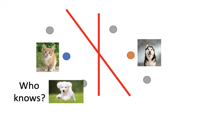
但如果有一些unlabeled data(如灰色的点),分类所画的boundary可能是一条斜线。
The distribution of the unlabeled data tell us something.
半监督式学习之所以有用,是因为这些unlabeled data的分布能告诉我们一些东西。
通常这也伴随着一些假设,所以半监督式学习是否有用往往取决于这些假设是否合理。
Semi-supervised Learning for Generative Model
Supervised Generative Model
在这篇文章中,有详细讲述分类问题中的generative model。
给定一个labelled training data $x^r\in C_1,C_2$ 训练集。
prior probability(先验概率)有 $P(C_i)$ 和 $P(x|C_i)$ ,假设是Gaussian模型,则 $P(x|C_i)$ 由Gaussian模型中的 $\mu^i,\Sigma$ 参数决定。
根据已有的labeled data,计算出假设的Gaussian模型的参数(如下图),从而得出prior probability。
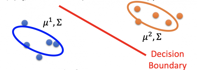
即可算出posterior probability $P\left(C_{1} \mid x\right)=\frac{P\left(x \mid C_{1}\right) P\left(C_{1}\right)}{P\left(x \mid C_{1}\right) P\left(C_{1}\right)+P\left(x \mid C_{2}\right) P\left(C_{2}\right)}$
Semi-supervised Generative Model
在只有labeled data的图中,算出来的 $\mu,\Sigma$ 参数如下图所示:
但如果有unlabeled data(绿色点),会发现分布的模型参数更可能是是下图:
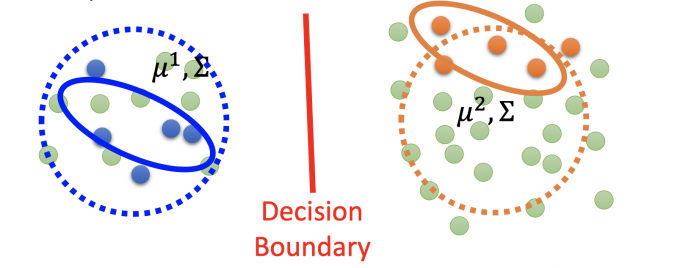
The unlabeled data $x^u$ help re-estimate $P(C_1),P(C_2),\mu^1,\mu^2,\Sigma$ .
因此,unlabeled data会影响分布,从而影响prior probability,posterior probability,最终影响 boundary。
EM
所以有unlabeled data, 这个Semi-supervised 的算法怎么做呢?
其实就是EM(Expected-maximization algorithm,期望最大化算法。)
Initialization : $\theta={P(C_1),P(C_2),\mu^1,\mu^2,\Sigma}$ .
初始化Gaussian模型参数,可以随机初始,也可以通过labeled data得出。
虽然这个算法最终会收敛,但是初始化的参数影响收敛结果,就像gradient descent一样。
E:Step 1: compute the posterior probability of unlabeled data $P_\theta(C_1|x^u)$ (depending on model $\theta$ )
根据当前model的参数,计算出unlabeled data的posterior probability $P(C_1|x^u)$ .(以$P(C_1|x^u)$ 为例)
M:Step 2: update model. Back to step1 until the algorithm converges enventually.
用E步得到unlabeled data的posterior probability来最大化极大似然函数,更新得到新的模型参数,公式很直觉。(以 $C_1$ 为例)
($N$ :data 的总数,包括unlabeled data; $N_1$ :label= $C_1$ 的data数)
$P(C_1)=\frac{N_1+\Sigma_{x^u}P(C_1|x^u)}{N}$
对比没有unlabeled data之前的式子, $P(C_1)=\frac{N_1}{N}$ ,除了已有label= $C_1$ ,还多了一部分,即unlabeled data中属于 $C_1$ 的概率和。
- $\mu^{1}=\frac{1}{N_{1}} \sum_{x^{r} \in C_{1}} x^{r}+\frac{1}{\sum_{x^{u}} P\left(C_{1} \mid x^{u}\right)} \sum_{x^{u}} P\left(C_{1} \mid x^{u}\right) x^{u}$
对比没有unlabeled data的式子 ,$\mu^{1}=\frac{1}{N_{1}} \sum_{x^{r} \in C_{1}} x^{r}$ ,除了已有的label= $C_1$ ,还多了一部分,即unlabeled data的 $x^u$ 的加权平均(权重为 $P(C_1\mid x^u)$ ,即属于 $C_1$ 的概率)。
$\Sigma$ 公式也包括了unlabeled data.
所以这个算法的Step 1就是EM算法的Expected期望部分,根据已有的labeled data得出极大似然函数的估计值;
Step 2就是EM算法的Maximum部分,利用unlabeled data(通过已有模型的参数)最大化E步的极大似然函数,更新模型参数。
最后反复迭代Step 1和Step 2,直至收敛。
Why EM
[1]挖坑EM详解。
为什么可以用EM算法来解决Semi-supervised?
只有labeled data
极大似然函数 $\log{L(\theta)}=\sum_{x^r}\log{P_\theta(x^r,\hat{y}^r)}$ , 其中 $P_\theta(x^r,\hat{y}^r)=P_\theta(x^r\mid \hat{y}^r)P(\hat{y}^r)$ .
对上式子求导是有closed-form solution的。
有labeled data和unlabeled data
极大似然函数增加了一部分 $\log L(\theta)=\sum_{x^{r}} \log P_{\theta}\left(x^{r}, \hat{y}^{r}\right)+\sum_{x^{u}} \log P_{\theta}\left(x^{u}\right)$ .
将后部分用全概率展开, $P_{\theta}\left(x^{u}\right)=P_{\theta}\left(x^{u} \mid C_{1}\right) P\left(C_{1}\right)+P_{\theta}\left(x^{u} \mid C_{2}\right) P\left(C_{2}\right)$ .
如果要求后部分,因为是unlabeled data, 所以模型 $\theta$ 需要得知unlabeled data的label,即 $P(C_1\mid x^u)$ ,而求这个式子,也需要得到 prior probability $P(x^u\mid C_1)$ ,但这个式子需要事先得知模型 $\theta$ ,因此陷入了死循环。
因此这个极大似然函数不是convex(凸),不能直接求解,因此用迭代的EM算法逐步maximum极大似然函数。
Low-density Separation Assumption
另一种假设是Low-density Separation的假设,即这个世界是非黑即白的”Black-or-white”。
两种类别之间是low-density,交界处有明显的鸿沟,因此要么是类别1,要么是类别2,没有第三种情况。
Self-training
对于Low-density Separation Assumption的假设,使用Self-training的方法。
Given:labeled data set $=\{(x^r,\hat{y}^r\}_{r=1}^R$ ,unlabeled data set $ =\{x^u\}_{u=R}^{R+U}$ .
Repeat:
Train model $f^*$ from labeled data set. $f^*$ is independent to the model)
从labeled data set中训练出一个模型
Apply $f^*$ to the unlabeled data set. Obtain pseudo-label $\{(x^u,y^u\}_{u=l}^{R+U}\}$
用这个模型 $f^*$ 来预测unlabeled data set, 获得伪label
Remove a set of data from unlabeled data set, and add them into the labeled data set.
拿出一些unlabeled data(pseudo-label),放到labeled data set中,回到步骤1,再训练。
how to choose the data set remains open
如何选择unlabeled data 是自设计的
you can also provide a weight to each data.
训练中可以对unlabeled data(pseudo-label)和labeled data 赋予不同的权重.
注意: Regression模型是不能self-training的,因为unlabeled data和其pseudo-label放在模型中的loss为0,无法再minimize。
Hard Label
V.S. semi-supervised learning for generative model
Semi-supervised learning for generative model和Low-density Separation的区别其实是soft label 和hard label的区别。
Generative Model是利用来unlabeled data的 $P(C_1|x^u)$ posterior probability来计算新的prior probability,迭代更新模型。
而low-density是计算出unlabeled data的pseudo-label,选择性扩大labeled data set(即加入部分由pseudo-label的unlabeled data)来迭代训练模型。
因此,如果考虑Neural Network:
($\theta^*$ 是labeled data计算所得的network parameters)
如下图,unlabeled data $x^u$ 放入模型中预测,得到 $\begin{bmatrix} 0.7 \ 0.3\end{bmatrix}$ .
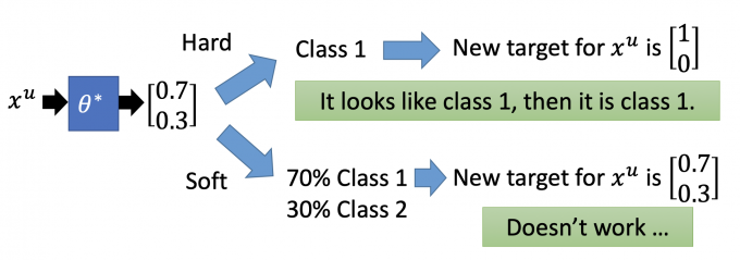
如果是使用hard label,则 $x^u$ 的target是 $\begin{bmatrix} 1 \ 0\end{bmatrix}$ .
如果是使用soft label,则 $x^u$ 的target是 $\begin{bmatrix} 0.7 \ 0.3\end{bmatrix}$ .
如果是使用soft label,则self-training不会有效,因为新的data对原loss的改变为0,不会增大模型的loss,也就无法再对其minimize.
所以基于Low-density Separation的假设,是非黑即白的,需要使用hard label来self-training。
Entropy-based Regularization
在训练模型中,我们需要尽量保证unlabeled data在模型中的分布是low-density separation。
即下图中,unlabeled data得到的pseudo-label的分布应该尽量集中,而不应该太分散。
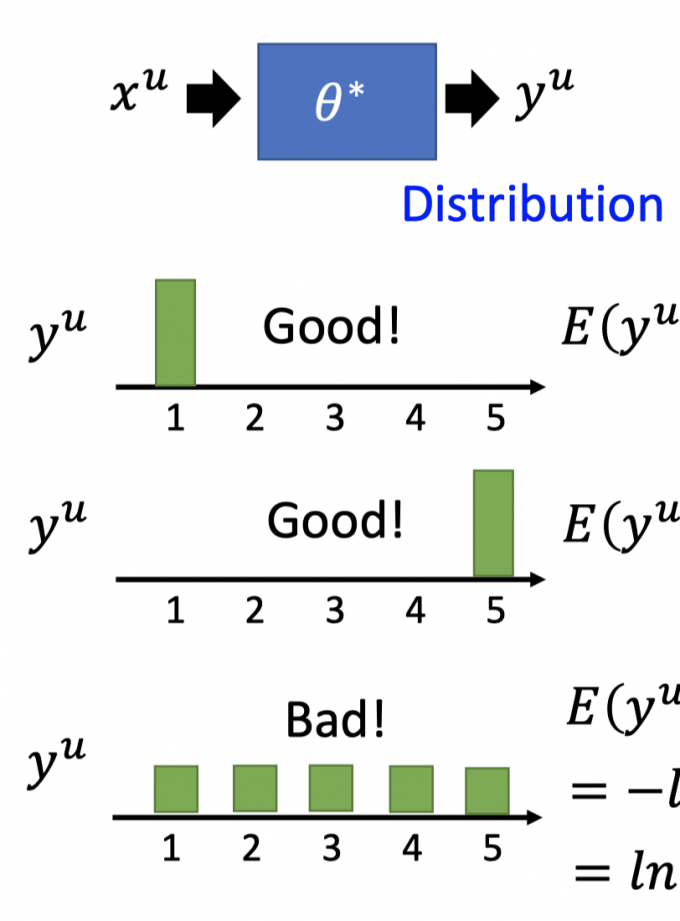
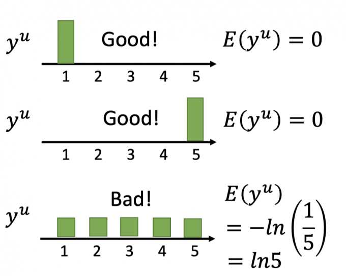
所以,在训练中,如何评估 $y^u$ 的分布的集中度?
根据信息学,使用 $y^u$ 的entropy,即 $E\left(y^{u}\right)=-\sum_{m=1}^{5} y_{m}^{u} \ln \left(y_{m}^{u}\right)$
(注:这里的 $y^u_m$ 是变量 $y^u=m$ 的概率)
当 $E(y^u)$ 越小,说明 $y^u$ 分布越集中,如下图。
因此,在self-training中:
$L=\sum_{y^r} C(x^r,\hat{y}^r)+\lambda\sum_{x^u}E(y^u)$
Loss function的前一项(cross entropy)minimize保证分类的正确性,后一项(entropy of $y^u$ ) minimize保证 unlabeled data分布尽量集中,最大可能满足low-density separation的假设。
training:gradient decent.
因为这样的形式很像之前提到过的regularization(具体见这篇文章的3.2),所以又叫entropy-based regularization.
Outlook: Semi-supervised SVM
SVM也是解决semi-supervised learning的方法.
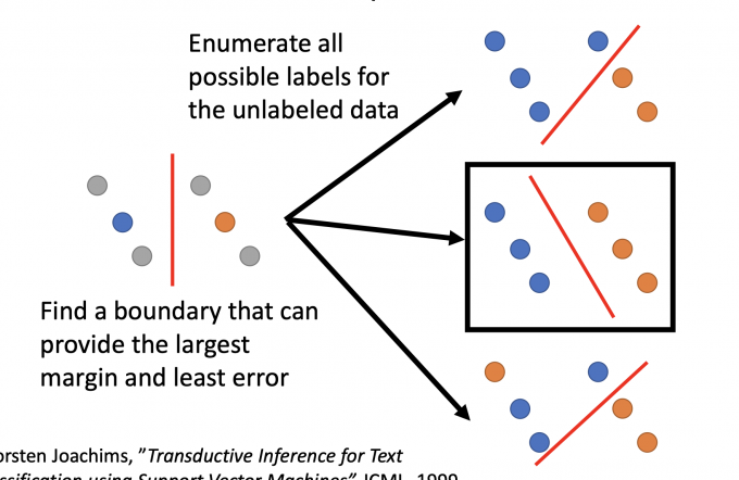
上图中,在有unlabeled data的情况下,希望boundary 分的越开越好(largest margin)和有更小的error.
因此枚举unlabeled data所有可能的情况,但枚举在计算量上是巨大的,因此SVM(Support Vector Machines)可以实现枚举的目标,但不需要这么大的枚举量。
Smoothness Assumption
Smoothness Assumption的思想可以用以下话归纳:
“You are known by the company you keep”
近朱者赤,近墨者黑。
蓬生麻中,不扶而直。白沙在涅,与之俱黑。
Assumption:“similar” $x$ has the same $\hat{y}$ .
【意思就是说:相近的 $x$ 有相同的label $\hat{y}$ .】
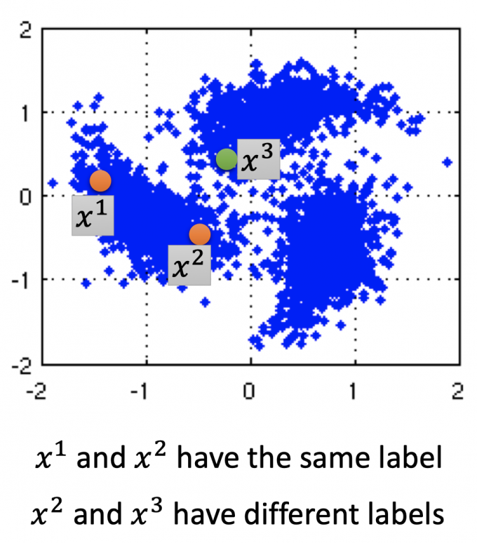
More precise assumption:
- x is not uniform
- if $x^1$ and $x^2$ are close in a hign density region, $\hat{y}^1$ and $\hat{y}^2$ are the same.
Smoothness Assumption假设更准确的表述是:
x不是均匀分布,如果 $x^1$ 和 $x^2$ 通过一个high density region的区域连在一起,且离得很近,则 $\hat{y}^1$ 和 $\hat{y}^2$ 相同。
如下图, $x^1$ 和 $x^2$ 通过high density region连接在一起,有相同的label,而 $x^2$ 和 $x^3$ 有不同的label.
Smoothness Assumption通过观察大量unlabeled data,可以得到一些信息。
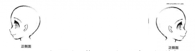
比如下图中的两张人的左脸和右脸图片,都是unlabeled,但如果给大量的过渡形态(左脸转向右脸)unlabeled data,可以得出这两张图片是相似的结论.
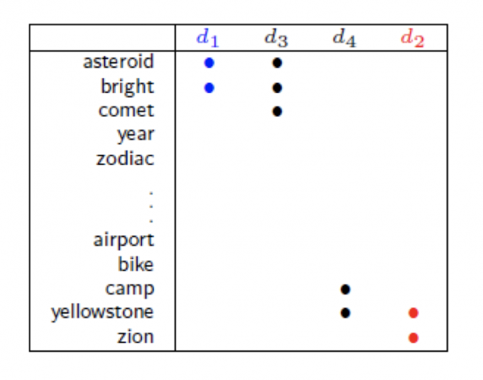
Smoothness Assumption还可以用在文章分类中,比如分类天文学和旅游学的文章。
如下图, 文章 d1和d3有overlap word(重叠单词),所以d1和d3是同一类,同理 d4和d2是一类。
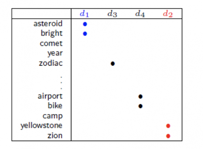
如果,下图中,d1和d3没有overlap word,就无法说明d1和d3是同一类。
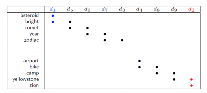
但是,如果我们收集到足够多但unlabeled data,如下图,通过high density region的连接和传递,也可以得出d1和d3一类,d2和d4一类。
Cluster and then Label
在Smoothness Assumption假设下,直观的可以用cluster and then label,先用所有的data训练一个classifier。
直接聚类标记(比较难训练)。
Graph-based Approach
另一种方法是利用图的结构(Graph structure)来得知 $x^1$ and $x^2$ are close in a high density region (connected by a high density path).
Represent the data points as a graph.
【把这些数据点看作一个图】
建图有些时候是很直观的,比如网页中的超链接,论文中的引用。
但有的时候也需要自己建图。
注意:
如果是影像类,base on pixel,performance就不太好,一般会base on autoencoder,将feature抽象出来,效果更好。
Graph Construction
建图过程如下:
Define the similarity $s(x^i, x^j)$ between $x^i$ and $x^j$ .
【定义data $x^i$ 和 $x^j$ 的相似度】
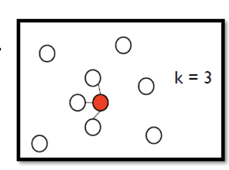
Add edge【定义数据点中加边(连通)的条件】
K Nearest Neighbor【和该点最近的k个点相连接】
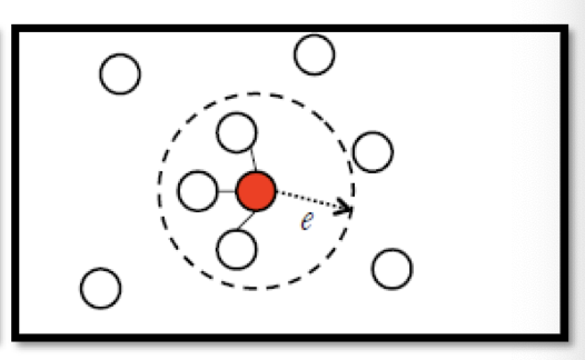
e-Neighborhood【与离该点距离小于等于e的点相连接】
Edge weight is proportional to $s(x^i, x^j)$ 【边点权重就是步骤1定义的连接两点的相似度】
Gaussian Radial Basis Function: $s\left(x^{i}, x^{j}\right)=\exp \left(-\gamma\left\|x^{i}-x^{j}\right\|^{2}\right)$
一般采用如上公式(经验上取得较好的performance)。
因为利用指数化后(指数内是两点的Euclidean distance),函数下降的很快,只有当两点离的很近时,该相似度 $s(x^i,x^j)$ 才大,其他时候都趋近于0.
Graph-based Approach
图建好后:
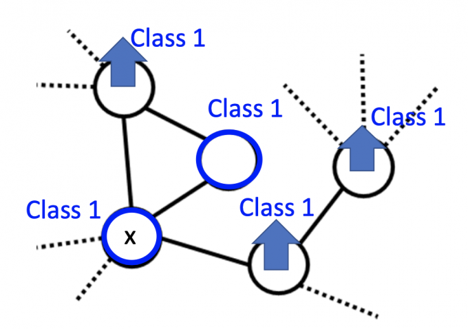
The labeled data influence their neighbors.
Propagate through the graph.
【label data 不仅会影响他们的邻居,还会一直传播下去】
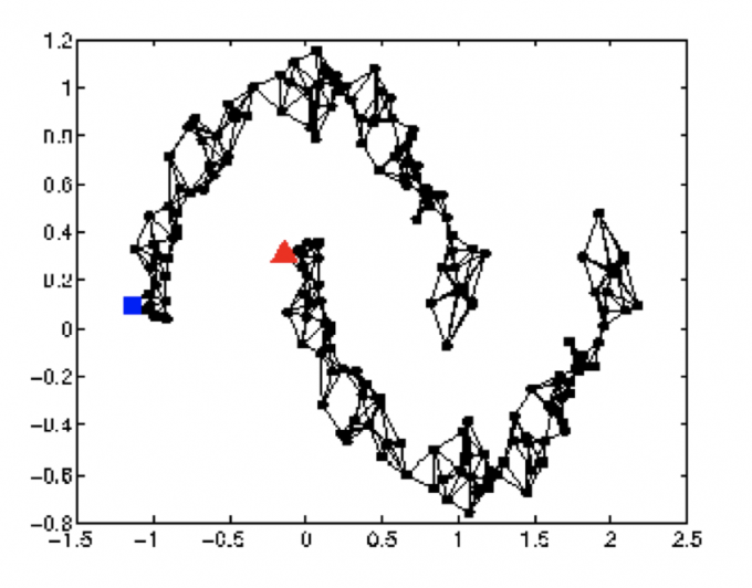
如果data points够多,图建的好,就会像下图这样:
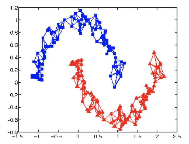
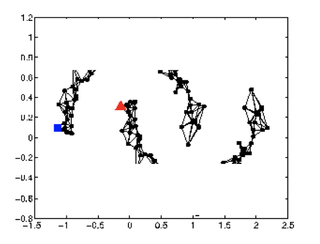
但是,如果data较少,就可能出现下图这种label传不到unlabeled data的情况:
Smoothness Definition
因为是基于Smoothness Assumption,所以最后训练出的模型应让得到的图尽可能满足smoothness的假设。
注意: 这里的因果关系是,unlabeled data作为NN的输入,得到label $y$ ,该label $y$ 和labeled data的 label $\hat{y}$ 一起得到的图是尽最大可能满足Smoothness Assumption的。
(而不是建好图,然后unlabeled data的label $y$ 是labeled data原有的 $\hat{y}$ 直接传播过来的,不然训练NN干嘛)
把unlabeled data作为NN的输入,得到label ,对labeled data和”unlabeled data” 建图。
为了在训练中使得最后的图尽可能满足假设,定义smoothness of the labels on the graph.
$S=\frac{1}{2} \sum_{i,j} w_{i, j}\left(y^{i}-y^{j}\right)^{2}$(对于所有的labeled data 和 “unlabeled data”(作为NN输入后,有label))
按照上式计算,得到的Smoothness如下图所示:
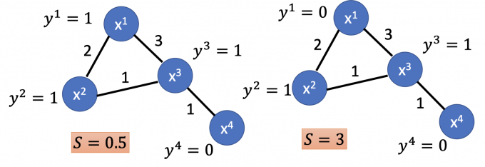
Smaller means smoother.
【Smoothness $S$ 越小,表示图越满足这个假设】
计算smoothness $S$ 有一种简便的方法:
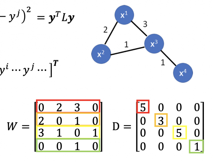
$S=\frac{1}{2} \sum_{i, j} w_{i, j}\left(y^{i}-y^{j}\right)^{2}=y^{T} L y$ (这里的1/2只是为了计算方便)$y$ : (R+U)-dim vector,是所有label data和”unlabeled data” 的label,所以是R+U维。
$y=\begin{bmatrix}…y^i…y^j…\end{bmatrix}^T$
$L$ :(R+U) $\times$ (R+U) matrix,也叫Graph Laplacian(调和矩阵,拉普拉斯矩阵)
$L$ 的计算方法:$L=D-W$
其中 $W$ 矩阵算是图的邻接矩阵(区别是无直接可达边的值是0)
$D$ 矩阵是一个对角矩阵,对角元素的值等于 $W$ 矩阵对应行的元素和
矩阵表示如下图所示:
(证明据说很枯燥,暂时略[2])
Smoothness Regularization
$S=\frac{1}{2} \sum_{i, j} w_{i, j}\left(y^{i}-y^{j}\right)^{2}=y^{T} L y$$S$ 中的 $y$ 其实是和network parameters有关的(unlabeled data的label),所以把 $S$ 也放进损失函数中minimize,以求尽可能满足smoothness assumption.
以满足smoothness assumption的损失函数: $L=\sum_{x^r} C\left(y^{r}, \hat{y}^{r}\right)+\lambda S$
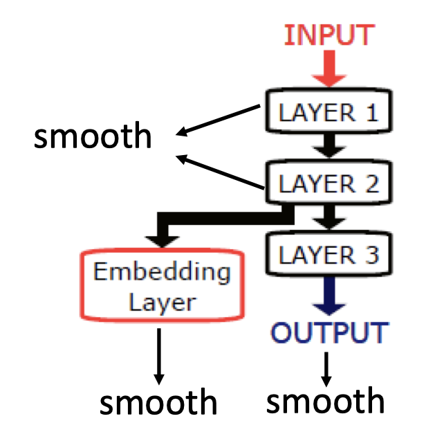
损失函数的前部分使labeled data的输出更贴近其label,后部分 $\lambda S$ 作为regularization term,使得labeled data和unlabeled data尽可能满足smoothness assumption.
除了让NN的output满足smoothness的假设,还可以让NN的任何一层的输出满足smoothness assumption,或者让某层外接一层embedding layer,使其满足smoothness assumption,如下图:
Better Representation
Better Presentation的思想就是:去芜存菁,化繁为简。
- Find the latent(潜在的) factors behind the observation.
- The latent factors (usually simpler) are better representation.
【找到所观察事物的潜在特征,即该事物的better representation】
该部分后续见这篇博客。
Reference
挖坑:EM算法详解
挖坑:Graph Laplacian in smoothness.
Olivier Chapelle:Semi-Supervised Learning
「机器学习-李宏毅」:Semi-supervised Learning