「Cryptography-ZKP」: Lec4-SNARKs via IP

In this series, I will learn Zero Knowledge Proofs (ZKP) on this MOOC, lectured by Dan Boneh, Shafi Goldwasser, Dawn Song, Justin Thaler and Yupeng Zhang.
Any corrections and advice are welcome. ^ - ^

Topics:

• Differences between Interactive Proofs and SNARKs
• Outline of SNARKs from IP
• Brief intro to Functional Commitments
• SZDL Lemma
• Multilinear Extensions
• Sum-check Protocol and its application.
  • Counting Triangles
  • SNARK for Circuit-satisfiability

Before proceeding to today’s topic, let’s briefly recall what is a SNARK?

• SNARK is a succinct proof that a certain statement is true.
  For example, such a statement could be “I know an m such that SHA256(m)=0”.
• SNARK indicates that the proof is “short” and “fast” to verify.
  Note that if m is 1GB then the trivial proof, i.e. the message m, is neither short nor fast to verify.

Interactive Proofs: Motivation and Model

In traditional outsourcing, the Cloud Provider stores the user’s data and the user can ask the Cloud Provider to run some program on its data. The user just blindly trusts the answer returned by the Cloud Provider.

The motivation for Interactive Proofs (IP) is that the above procedure can be turned into the following Challenge-Response procedure. The user is allowed to send a challenge to the Cloud Provider and the Cloud Provider is required to respond for such a challenge.

The user has to accept if the response is valid or reject as invalid.

Hence, the Challenge-Response procedure or IP can be modeled as follows.

• P solves a problem and tells V the answer.
  • Then they have a conversation.
  • P’s goal is to convince V that the answer is correct.
• Requirements:
  1. Completeness: an honest P can convince V to accept the answer.
  2. (Statistical) Soundness: V will catch a lying P with high probability.

Note that statistical soundness is information-theoretically soundness so IPs are not based on cryptographic assumptions.

Hence, the soundness must hold even if P is computationally unbounded and trying to trick V into accepting the incorrect answer.

If soundness holds only against polynomial-time provers, then the protocol is called an interactive argument.

It is worth noting that SNARKs are arguments so it is not statistically sound.

IPs v.s. SNARKs

There are three main differences between Interactive Proofs and SNARKs. We’ll list them first and elaborate in the section.

1. SNARKs are not statistically sound.
2. SNARKs have knowledge soundness.
3. SNARKs are non-interactive.

Not Statistically Sound

The first one is mentioned above that SNARKs are arguments so the soundness is only against polynomial-time provers.

Knowledge Soundness v.s. Soundness

The second one is that SNARKs has knowledge soundness.

SNARKs that don’t have knowledge soundness are called SNARGs, they are studied too.

Considering a public arithmetic circuit such that $C(x,w)=0$ where $x$ is the public statement and $w$ is the secret witness.

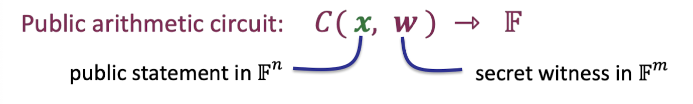
Compare soundness to knowledge soundness for such a circuit-satisfiability.

• Sound: V accepts → There exist $w$ s.t. $C(x,w)=0$.
• Knowledge sound: V accepts → P actually “knows” $w$ s.t. $C(x,w)=0$.
  The prover is establishing that he necessarily knows the witness.

As for the soundness, the prover is only establishing the existence of such a witness.

The knowledge soundness is establishing that the prover necessarily knows the witness.

Hence, knowledge soundness is stronger.

But sometimes standard soundness is meaningful even in contexts where knowledge soundness isn’t, and vice versa.

• Standard soundness is meaningful.
  • Because there’s no natural “witness”.
  • E.g., P claims the output of V’s program on $x$ is 42.
• Knowledge soundness is meaningful.
  • E.g., P claims to know the secret key that controls a certain Bitcoin wallet.
  • It is actually claimed that the prover knows a pre-image such that the hash is 0.
  • The hash function is surjective so a witness for this claim always exists. In fact, there are many and many witnesses for this claim. It turns to a trivial sound protocol.
  • Hence, it needs to establish that the prover necessarily knows the witness.

Non-interactive and Public Verifiability

The final difference is that SNARKs are non-interactive.

Interactive proof and arguments only convince the party that is choosing or sending the random challenges.

This is bad if there are many verifiers as in most blockchain applications. P would have to convince each verifier separately.

For public coin protocols, we have a solution, Fiat-Shamir, which renders the protocol non-interactive and publicly verifiable.

In quiz 4, it is a false statement that non-interactive implies publicly verifiable.

In my perspective, it only holds for non-interactive protocols rendered from the public coin protocols where the verifier only sample random coins and send the sampled coins to the provers.

SNARKs from Interactive Proofs: Outline

We’ll describe the outline to build SNARKs from interactive proofs in this section.

Trivial SNARKs

The first thing to point out is that the trivial SNARK is not a SNARK.

The trivial SNARK is as follows:

1. Prover sends $w$ to verifier.
2. Verifier checks if $C(x,w)=0$ and accepts if so.
   The verifier is required to rerun the circuit.

The above trivial SNARK has two problems:

• The witness $w$ might be long.
  • We want a “short” proof $\pi$ → $\text{len}(\pi)=\text{sublinear}(|w|)$
• Computing $C(x,w)$ may be hard.
  • We want a “fast” verifier → $\text{time}(V)=O_\lambda(|x|, \text{sublinear(|C|)})$.

As described in Lecture 2, succinctness means the proof length is sublinear in the length of the witness and the verification time is linear to the length of public statement $x$ and sublinear to the size of the circuit $C$. Note that the verification time linear to $|x|$ means that the verifier at least read the statement $x$.

Less Trivial

We can make it less trivial as follows:

1. Prover sends $w$ to verifier.
2. Prover uses an IP to prove that $w$ satisfies the claimed property.

It gives a fast verifier, but the proof is still too long.

Actual SNARKs

In actual SNARKs, instead of sending $w$, the prover commits cryptographically to $w$.

Consequently, the actual SNARKs is described as follows:

1. Prover commits cryptographically to $w$.
2. Prover uses an IP to prove that $w$ satisfies the claimed property.

The IP procedure reveals just enough information about the committed witness $w$ to allow the verifier to run its checks.

Moreover, the IP procedure can be rendered non-interactive via Fiat-Shamir.

Functional Commitments

There are several important functional families introduced in Lecture 2 we want to build commitment schemes.

• Polynomial commitments: commit to a univariate $f(X)$ in $\mathbb{F}_p^{(\le d)}[X]$.
  $f(X)$ is a univariate polynomial in the variable $X$ that has a degree at most $d$.

  1. The prover commits to a univariate polynomial of degree $\le d$ .

  2. Later the verifier requests to know the evaluation of this polynomial at a specific point $r$.

  3. The prover can reveal $f(r)$ and provide proof that the revealed evaluation is consistent with the committed polynomial.

     Note that the proof size and verifier time should be $O_\lambda(\log d)$ in SNARKs.

• Multilinear commitments: commit to multilinear $f$ in $\mathbb{F}_p^{(\le 1)}[X_1,\dots, X_k]$.
  $f$ is a multilinear polynomial in variables $X_1,\dots, X_k$ where each variable has a degree at most 1. E.g., $f(x_1,\dots, x_k)=x_1x_3 + x_1 x_4 x_5+x_7$.

• Vector commitments (e.g. Merkle trees): commit to a vector $\vec{u}=(u_1,\dots, u_d)\in \mathbb{F}_p^d$.

  1. The prover commits to a vector of $d$ entries.
  2. Later the verifier requests the prover to open a specific entry of the vector, e.g. the $i$th entry $f_{\vec{u}}(i)$.
  3. The prover can open the $i$th entry $f_{\vec{u}}(i)=u_i$ and provide a short proof that the revealed entry is consistent with the committed vector.

• Inner product commitments (inner product arguments - IPA): commit to a vector $\vec{u}=(u_1,\dots, u_d)\in \mathbb{F}_p^d$.

  1. The prover commits to a vector $\vec{u}$.
  2. Later the verifier requests the prover to open an inner product $f_{\vec{u}}(\vec{v})$ that takes a vector $\vec{v}$ as input.
  3. The prover can open the inner product $f_{\vec{u}}(\vec{v})=(\vec{u},\vec{v})$ and provide a short proof that the revealed inner product is consistent with the committed vector.

Vector Commitments: Merkle Trees

In vector commitments, the prover wants to commit a vector.

We can pair up the values in the vector and hash them to form a binary tree.

A Merkle tree is a binary tree where the leaf node stores the values of the vector that we want to commit and the other internal nodes calculate the hash value of its two children nodes.

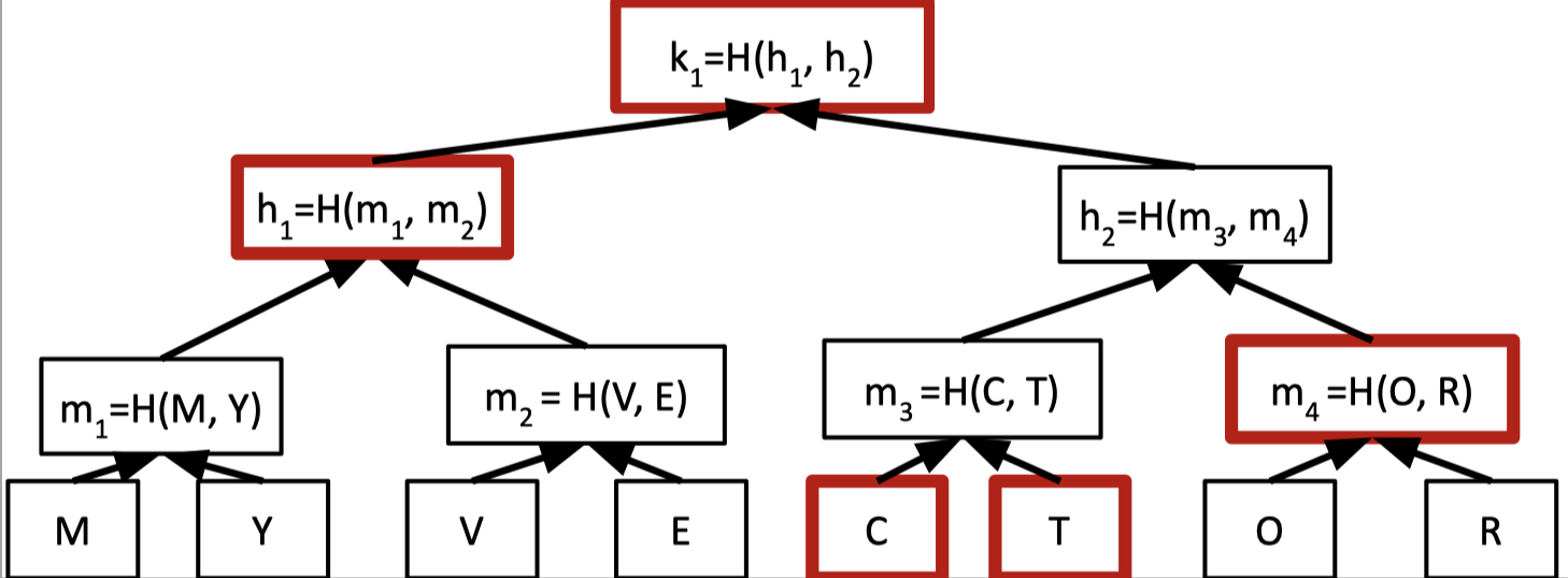
The root hash is the commitment of the vector so the prover just sends the root hash to the verifier as the commitment.

Then the verifier wants to know the 6th entry in the vector.

The prover provides the 6th entry (T) and proof that the revealed entry is consistent with the committed vector. The proof is also called the authentication information.

The authentication information is the sibling hashes of all nodes on the root-to-leaf path that includes $C, m_4, h_1$. Hence, the proof size is $O(\log n)$ hash values.

The verifier can check these hashes are consistent with the root hash.

Under the assumption that $H$ is a collision-resistant hash family, the vector commitment has the binding property that once the root hash is sent, the committer is bound to a fixed vector.

Because opening any leaf to two different values requires finding a hash collision along the root-to-leaf path.

Poly Commitments via Merkle Trees

A natural way of constructing polynomial commitments is to use the Merkle trees.

For example, we can commit to a univariate $f(X)$ in $\mathbb{F}_7^{(\le d)}[X]$ with the following Merkle tree.

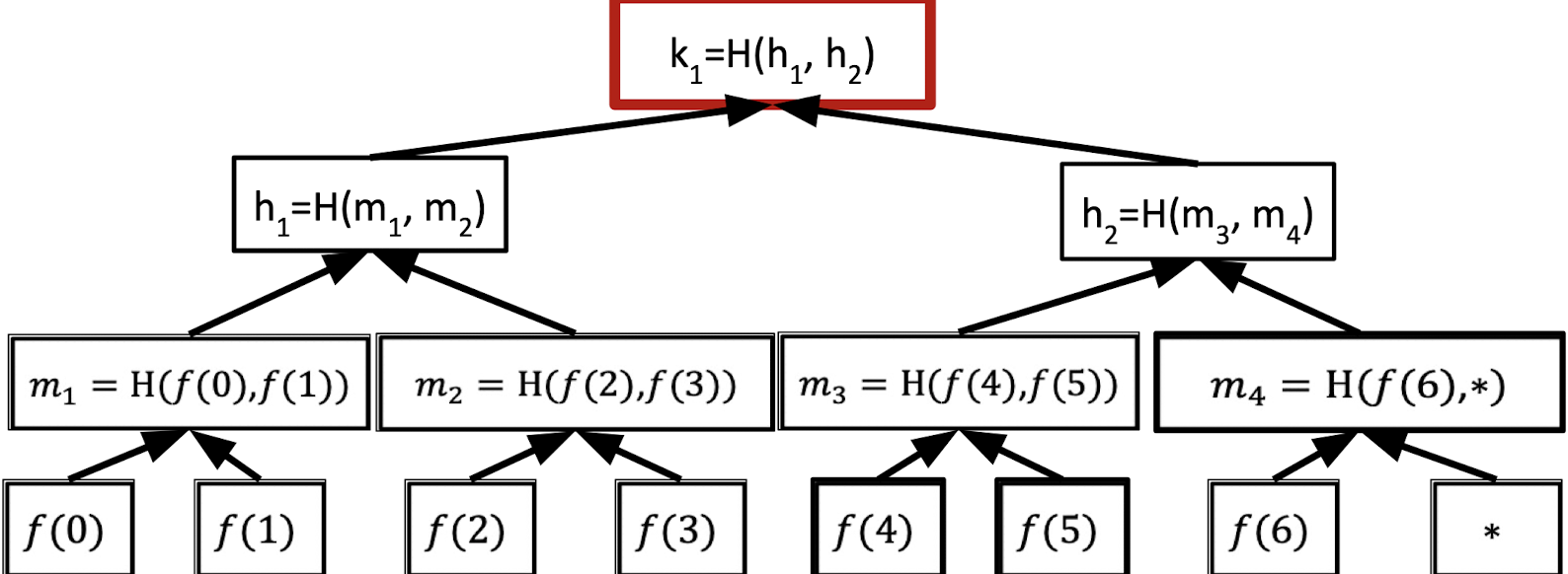
When the verifier requests to reveal $f(4)$, the prover can provide $f(4)$ and the following sibling hashes as proof.

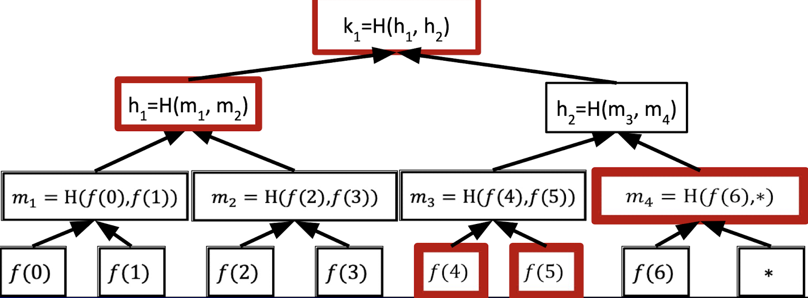
In summary, if we want to commit a univariate $f(X)$ in $\mathbb{F}^{(\le d)}[X]$, the prover needs to Mekle-commit to all evaluations of the polynomial $f$.

When the verifier requests $f(r)$, the prover reveals the associated leaf along with opening information.

However, it has two problems.

• The number of leaves is $|\mathbb{F}|$ which means the time to compute the commitment is at least $|\mathbb{F}|$. It is a big problem when working over large fields, e.g., $|\mathbb{F}|\approx 2^{64}$ or $|\mathbb{F}|\approx 2^{128}$.
  → We want the time proportional to the degree bound $d$.
• The verifier does not know if $f$ has a degree at most $d$ !.

In lecture 5, we will introduce KZG polynomial commitment scheme using bilinear groups, which addresses both issues.

Tech Preliminaries

SZDL Lemma

The heart of IP design is based on a simple observation.

For a non-zero $f\in \mathbb{F}_p^{(\le d)}[X]$, if we sample a random $r$ from the field $\mathbb{F}_p$, the probability of $f(r)=0$ is at most $d/p$.

Suppose $p\approx 2^{256}$ and $d\le 2^{40}$, then $d/p$ is negligible.

If $f(r)=0$ for a random $r\in \mathbb{F}_p$, then $f$ is identically zero w.h.p.

It gives us a simple zero test for a committed polynomial.

Moreover, we can achieve a simple equality test for two committed polynomials.

Let $p,q$ be univariate polynomials of degree at most $d$. Then $\operatorname{Pr}_{r\overset{\$}\leftarrow \mathbb{F}}[p(r)=q(r)]\le d/p$.

If $f(r)=g(r)$ for a random $\overset{\$}\leftarrow \mathbb{F}_p$, then $f=g$ w.h.p.

The Schwartz-Zippel-Demillo-Lipton lemma is a multivariate generalization of the above facts.

Schwartz-Zippel-Demillo-Lipton Lemma (SZDL Lemma):

Let $p,q$ be $\ell$-variate polynomials of total degree at most $d$. Then $\operatorname{Pr}_{r\in \mathbb{F}^{\ell}}[p(r)=q(r)]\le d/{|\mathbb{F}|}$.

”Total degree” refers to the maximum sum of degree of all variables in any term.

Low-Degree and Multilinear Extensions

Using many variables, we are able to keep the total degree of polynomials quite low, which ensures the proof is short and fast to verify.

Definition of Polynomial Extensions:

Given a function $f:\{0,1\}^{\ell}\rightarrow \mathbb{F}$, a $\ell$-variate polynomial $g$ over $\mathbb{F}$ is said to extend $f$ if $f(x)=g(x)$ for all $x\in \{0,1\}^{\ell}$.

Note that the original domain of $f$ is $\{0,1\}^{\ell}$ and the domain of extension $g$ is much bigger, that’s $\mathbb{F}^{\ell}$.

Definition of Multilinear Extensions:

Any function $f:\{0,1\}^{\ell}\rightarrow \mathbb{F}$ has a unique multilinear extension (MLE) denoted by $\tilde{f}$.

The total degree of the multilinear extension can be vastly smaller than the degree of the original univariate polynomial.

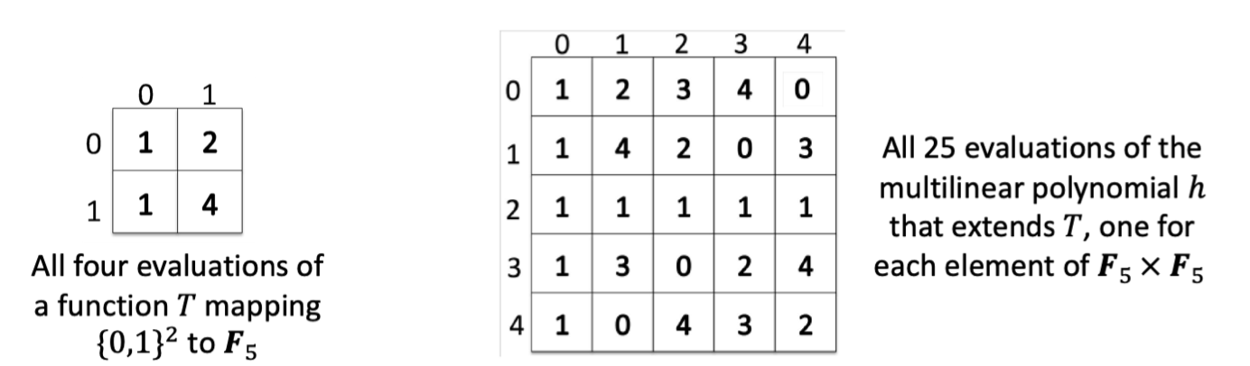
Consider a univariate polynomial $f:\{0,1\}^2\rightarrow \mathbb{F}$ as follows. It maps $00$ to $1$, maps $01$ to 2, and so on.

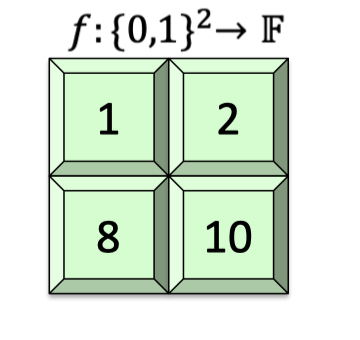
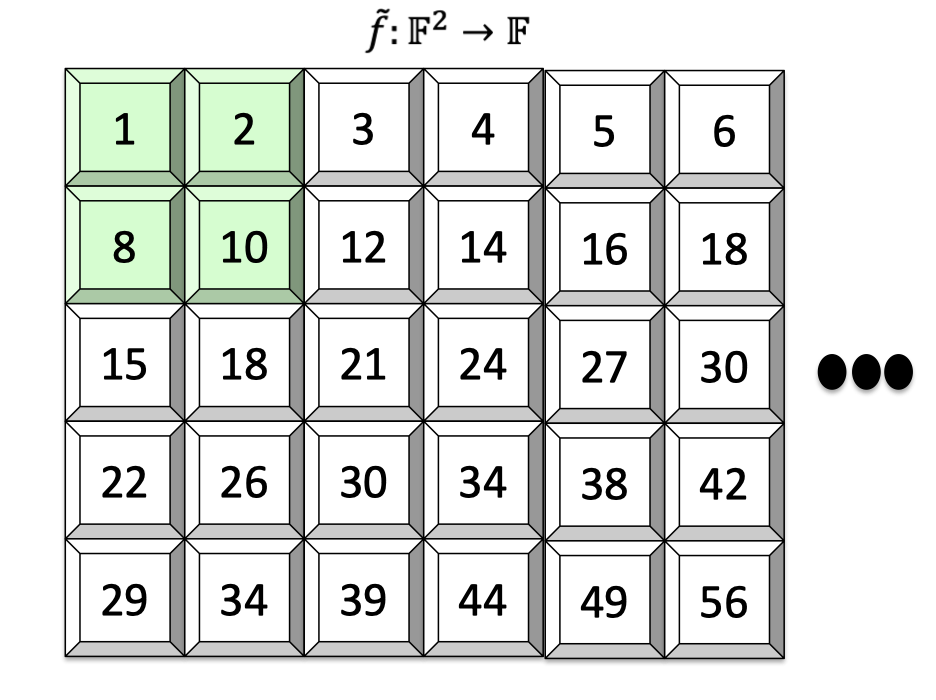
The multilinear extension $\tilde{f}:\mathbb{F}^2\rightarrow \mathbb{F}$ is defined as $\tilde{f}(x_1,x_2)=(1-x_1)(1-x_2)+2(1-x_1)x_2+8x_1(1-x_2)+10x_1x_2$.

Its domain is field by field and it’s easy to check that $\tilde{f}(0,0)=1,\tilde{f}(0,1)=2,\tilde{f}(1,0)=8$ and $\tilde{f}(1,1)=10$.

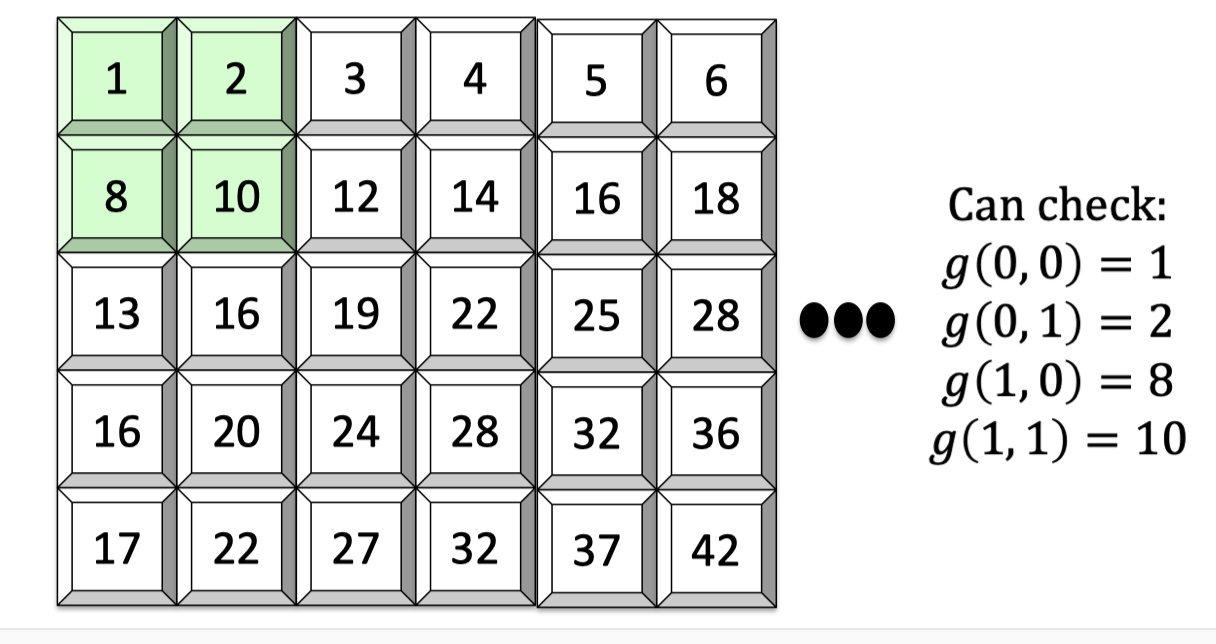
Another non-multilinear extension of $f$ could be defined as $g(x_1,x_2)=-x_1^2+x_1x_2+8x_1+x_2+1$.

Evaluating multilinear extensions quickly

The sketch of evaluating the multilinear extension is Lagrange interpolation.

Fact:

Given as input all $2^{\ell}$ evaluations of a function $f:\{0,1\}^\ell \rightarrow \mathbb{F}$, for any point $r\in \mathbb{F}^{\ell}$, there is an $O(2^{\ell})$-time algorithm for evaluating $\tilde{f}(r)$.

Algorithm:

• Define $\tilde{\delta}_w(r)=\prod_{i=1}^\ell (r_iw_i+(1-r_i)(1-w_i)).$

  This is called the multilinear Lagrange basis polynomial corresponding to $w$.

  For any input $r$, $\tilde{\delta}_w(r)=1$ if $r=w$, and $0$ otherwise.

• Hence, we can evaluate the multilinear extension of any input $r$ as follows.

  $$ \tilde{f}(r)=\sum_{w\in \{0,1\}^\ell}f(w)\cdot \tilde{\delta}_w(r) $$

• Complexity: For each $w\in \{0,1\}^{\ell}$, $\tilde{\delta}_w(r)$ can be computed with $O(\ell)$ field operations, which yields an $O(\ell 2^\ell)$-time algorithm.

  It can be reduced to time $O(2^\ell)$ via dynamic programming.

If we feed this algorithm with the description of $f$ whose domain is $\{0,1\}^\ell$ as inputs and the description consists of all $2^\ell$ evaluations of $f$, then it is possible to evaluate the multilinear extension of $f$ at any desired point.

This fact means that evaluating multilinear extension is essentially as fast as $O(2^\ell)$, which is constantly slower than reading the whole description of $f$.

The Sum-Check Protocol

In this part, we’ll introduce the sum-check protocol [Lund-Fortnow-Karloff-Nissan’90].

We have a verifier with an oracle access to a $\ell$-variate polynomial $g$ over field $\mathbb{F}$. The verifier’s goal is to compute the following quantity:

$$ \sum_{b_1\in\{0,1\}}\sum_{b_2\in\{0,1\}}\dots \sum_{b_\ell\in\{0,1\}} g(b_1,\dots, b_\ell) $$

As described above (functional commitments), the prover commit a multilinear polynomial, later the verifier can request the prover to evaluate at some specific points. Then the prover provide the evaluation and the proof that the revealed evaluation is consistent with the committed polynomial.

In this part, we consider this process as a black box or an oracle. The verifier can go to the oracle and requests the evaluation of $g$ at some points.

Note that this sum is the sum of all $g$’s evaluations over inputs $\{0,1\}^\ell$ so the verifier can compute it on his own by just asking the oracle for the evaluations. But it costs the verifier $2^\ell$ oracle queries.

Protocol

Instead, we can offload the work of the verifier to the prover where the prover computes the sum and convince the verifier that the sum is correct.

It turns out that the verifier only have to run $\ell$-rounds to check the prover’s answer with only $1$ oracle query.

Denote $P$ as prover and $V$ as verifier.

Let’s dive into the start phase and the first round.

• Start: $P$ sends claimed answer $C_1$. The protocol must check that:

  $C_1=\sum_{b_1\in\{0,1\}}\sum_{b_2\in\{0,1\}}\dots \sum_{b_\ell\in\{0,1\}} g(b_1,\dots, b_\ell)$

• Round 1: $P$ sends a univariate polynomial $s_1(X_1)$ claimed to equal:

  $H_1(X_1):=\sum_{b_2\in\{0,1\}}\dots \sum_{b_\ell\in\{0,1\}} g(X_1,\dots, b_\ell)$
  • $V$ checks that $C_1=s_1(0)+s_1(1)$.
    • If this check passes, it is safe for $V$ to believe that $C_1$ is the correct answer as long as $V$ believes that $s_1=H_1$.
    • It can be checked that $s_1$ and $H_1$ agree at a random point $r_1\in \mathbb{F}_p$ by SZDL lemma.
  • $V$ picks $r_1$ at random from $\mathbb{F}$ and sends $r_1$ to $P$.

In round 1, $s_1(X_1)$ is the univariate polynomial that prover actually sends while $H_1(X_1)$ is what the prover claim to send if the prover is honest.

Note that $H_1(X_1)$ is the true answer except that we cut off the first sum, which leave the first variable free. It reduce $2^\ell$ terms to $2^{\ell-1}$ terms.

$g$ is supposed to have low degree (2 or 3) in each variable so the univariate polynomial $H_1$ derived from $g$ has low degree.

Note: We can benefit from the low degree of the univariate polynomial. One is that specifying $H_1$ can be done by just sending 2 or 3 coefficients. Moreover, the low degree gives us acceptable or negligible sound error.

After receiving the $s_1$, $V$ can compute $s_1(r_1)$ directly, but not $H_1(r_1)$.

It turns out that $P$ can compute $H_1(r_1)$ and sends claimed $H_1(r_1)$ where $H_1(r_1)$ is the sum of $2^{\ell-1}$ terms where $r_1$ is fixed so the first variable in $g$ is bound to $r_1\in \mathbb{F}$.

$$ H_1(r_1):=\sum_{b_2\in\{0,1\}}\dots \sum_{b_\ell\in\{0,1\}} g(r_1,b_2,\dots, b_\ell) $$

Hence, the round 2 is indeed a recursive sub-protocol that checks $s_1(r_1)=H_1(r_1)$ where $s_1(r_1)$ is computed on $V$’s own.

• Round 2: They recursively check that $s_1(r_1)=H_1(r_1)$, i.e. that

  $$ s_1(r_1)=\sum_{b_2\in\{0,1\}}\dots \sum_{b_\ell\in\{0,1\}} g(r_1,b_2,\dots, b_\ell) $$

  • $P$ sends univariate polynomial $s_2(X_2)$ claimed to equal:

    $$ H_2(X_1):=\sum_{b_3\in\{0,1\}}\dots \sum_{b_\ell\in\{0,1\}} g(r_1,X_2,\dots, b_\ell) $$

  • $V$ checks that $s_1(r_1)=s_2(0)+s_2(1)$.

    • If this check passes, it is safe for $V$ to believe that $s_1(r_1)$ is the correct answer as long as $V$ believes that $s_2=H_2$.
    • It can be checked that $s_2$ and $H_2$ agree at a random point $r_2\in \mathbb{F}_p$ by SZDL lemma.

  • $V$ picks $r_2$ at random from $\mathbb{F}$ and sends $r_2$ to $P$.

• Round $i$: They recursively check that

  $$ s_{i-1}(r_{i-1})=\sum_{b_i\in\{0,1\}}\dots \sum_{b_\ell\in\{0,1\}} g(r_1,\dots,r_{i-1},b_i,\dots b_\ell) $$

  • $P$ sends univariate polynomial $s_i(X_i)$ claimed to equal:

    $$ H_i(X_i):=\sum_{b_{i+1}\in\{0,1\}}\dots \sum_{b_\ell\in\{0,1\}} g(r_1,\dots,r_{i-1},X_i,\dots b_\ell) $$

  • $V$ checks that $s_{i-1}(r_{i-1})=s_i(0)+s_i(1)$.

  • $V$ picks $r_i$ at random from $\mathbb{F}$ and sends $r_i$ to $P$.

• Round $\ell$: (Final round): They recursively check that

  $$ s_{\ell-1}(r_{\ell-1})= \sum_{b_\ell\in\{0,1\}} g(r_1,\dots,r_{\ell-1},b_\ell) $$

  • $P$ sends univariate polynomial $s_{\ell}(X_\ell)$ claimed to equal :

    $$ H_\ell(X_\ell):= g(r_1,\dots,r_{\ell-1},X_\ell) $$

  • $V$ checks that $s_{\ell-1}(r_{\ell-1})=s_\ell(0)+s_\ell(1)$.

  • $V$ picks $r_\ell$ at random, and needs to check that $s_\ell(r_\ell)=g(r_1,\dots,r_\ell)$.

    • No need for more rounds. $V$ can perform this check with one oracle query.

Consequently, the final claim that the verifier is left to check $s_\ell(r_\ell)=g(r_1,\dots,r_\ell)$ where $s_\ell(r_\ell)$ can be computed on its own and $g(r_1,\dots, r_\ell)$ can be computed with just a single query to the oracle.

If the final checks passes, then the verifier is convinced that $s_\ell(r_\ell)=g(r_1,\dots,r_\ell)$ and recursively convinced the claims left in the previous rounds, i.e. $s_i=H_i$. Finally, the verifier accepts the first claim that $C_1$ is the correct sum.

Analysis

Completeness:

Completeness holds by design. If $P$ sends the prescribed message, then all of $V$’s checks will pass.

Soundness:

If $P$ dose not send the prescribed messages, then $V$ rejects with probability at least $1-\frac{\ell\cdot d}{|\mathbb{F}|}$, where $d$ is the maximum degree of $g$ in any variable.

Proof of Soundness (Non-Inductive):

It is conducted by the union bound.

Specifically, if $C_1\ne \sum_{(b_1,\dots, b_\ell)\in \{0,1\}^{\ell}}g(b_1,\dots, b_\ell)$, then the only way the prover convince the verifier to accept is if there at least one round $i$ such that the prover sends a univariate polynomial $s_i(X_i)$ that dose not equal the prescribed polynomial

$$ H_i(X_i)=\sum_{(b_{i+1},\dots, b_\ell)}g(r_1, r_2,\dots, X_i,b_{i+1},\dots, b_\ell) $$

yet $s_i(r_i)=H_i(r_i)$.

For every round $i$, $s_i$ and $H_i$ both have degree at most $d$, and hence if $s_i\ne H_i$, then probability that $s_i(r_i)=H_i(r_i)$ is at most $d/|\mathbb{F}|$. By a union bound over all $\ell$ rounds, the probability that there (is a bad event) is any round $i$ such that the prover send a polynomial $s_i\ne H_i$ yet $s_i(r_i)=H_i(r_i)$ is at most $\frac{\ell\cdot d}{|\mathbb{F}|}$

Proof of Soundness by Induction:

• Base case: $\ell=1$.

  • In this case, $P$ sends a single message $s_1(X_1)$ claimed to equal $g(X_1)$.
  • $V$ picks $r_1$ at random, and checks $s_1(r_1)=g(r_1)$.
  • If $s_1\ne g$, then the probability that $s_1(r_1)=g(r_1)$ is at most $d/|\mathbb{F}|$.

• Inductive case: $\ell >1$.

  • Recall that $P$’s first message $s_1(X_1)$ is claimed to equal $H_1(X_1)$.
  • Then $V$ picks a random $r_1$ and sends $r_1$ to $P$. They recursively invoke sum-check to confirm $s_1(r_1)=H_1(r_1)$.
  • If $s_1\ne H_1$, then then probability that $s_1(r_1)=H_1(r_1)$ is at most $d/|\mathbb{F}|$.
  • Conditioned on $s_1(r_1)=H_1(r_1)$, $P$ is left to prove a false claim in the recursive call.
    • The recursive call applies sum-check to $g(r_1, X_2, \dots, X_\ell)$, which is $\ell-1$ variate.
    • By induction hypothesis, $P$ convinces $V$ in the recursive call with probability at most $\frac{d(\ell-1)}{|\mathbb{F}|}$.

• In summary, if $s_1\ne H_1$, the probability $V$ accepts is at most

  $$ \begin{aligned} \le &\operatorname{Pr}_{r_1\in \mathbb{F}}[s_1(r_1)=H_1(r_1)]+\operatorname{Pr}_{r_2,\dots, r_\ell\in \mathbb{F}}[V \text{ accepts}\mid s_1(r_1)\ne H_1(r_1)] \\ \le & \frac{d}{|\mathbb{F}|}+ \frac{d(\ell-1)}{|\mathbb{F}|}\le \frac{d\ell}{|\mathbb{F}|}\end{aligned} $$

Costs

Let $\mathrm{deg}_i(g)$ denote the degree of variable $X_i$ in $g$ and each variable has degree at most $d$.

$T$ denotes the time required to evaluate $g$ at one point.

• Total communication is $O(d\cdot \ell)$ field elements.

  • The total prover-to-verifier communication is $\sum_{i=1}^\ell(\mathrm{deg}_i(g)+1)=\ell+\sum_{i=1}^\ell \mathrm{deg}_i(g)=O(d\cdot \ell)$ field elements.
  • The total verifier-to-prover communication is $\ell-1$ field elements.

• Verifier’s runtime is $O(d\ell+T)$.

  • The running time of the verifier over the entire execution of the protocol is proportional to the total communication, plus the cost of a single oracle query to $g$ to compute $g(r_1,r_2, \dots, r_\ell)$.

• Prover’s runtime is $O(d\cdot 2^\ell\cdot T)$.
  Counting the number of evaluations over $g$ required by the prover is less straightforward.

  • In round $i$, $P$ is required to send a univariate polynomial $s_i$, which can be specified by $\mathrm{deg}_i(g)+1$ points.

  • Hence, $P$ can specify $s_i$ by sending for each $j\in {0, \dots, \mathrm{deg}_i(g)}$ the value:

    $$ s_i(j)=\sum_{(b_{i+1},\dots, b_\ell)}g(r_1,\dots,r_{i-1},j,b_{i+1},\dots, b_\ell) $$

  • An important insight is that the number of the terms defining $s_i(j)$ falls geometrically with $i$: in the $i$th sum, there are only $(1+\mathrm{deg}_i(g))\cdot 2^{\ell-i}\approx d\cdot 2^{\ell-i}$ terms, with the $2^{\ell-i}$ factor due to the number of vectors in $\{0,1\}^{\ell-i}$.

  • Thus, the total number of terms that must be evaluated is $\sum_{i=1}^\ell d\cdot 2^{\ell-i}=O(d\cdot 2^{\ell})$.

Application of Sum-check Protocol

An IP for counting triangles with linear-time verifier

The sum-check protocol can be applied to design an IP for counting triangles in a graph with linear-time verifier.

The input is an adjacent matrix of a graph $A\in \{0,1\}^{n\times n}$.

The desired output is $\sum_{(i,j,k)\in [n]^3}A_{ij}A_{jk}A_{ik}$, which counts the number of triangles in the graph.

The fastest known algorithm runs in matrix-multiplication time, currently about $n^{2.37}$, which is super linear time in the size of the matrix.

Likewise, we can offload the work to the prover to have a linear-time verifier.

To design an IP derived from sum-check protocol, we need to view the matrix $A$ to a function mapping $\{0,1\}^{\log n}\times \{0,1\}^{\log n}$ to $\mathbb{F}$.

It can be done easily by Lagrange interpolation. As for the following matrix $A\in \mathbb{F}^{4\times 4}$, we can interpret the entry location $(i,j)\in \{0,1\}^{\log n}\times \{0,1\}^{\log n}$ as input and maps to the corresponding value $A_{i,j}\in \mathbb{F}$. E.g., $A(0,0,0,0)=1,A(0,0,0,1)=3$ and so on.

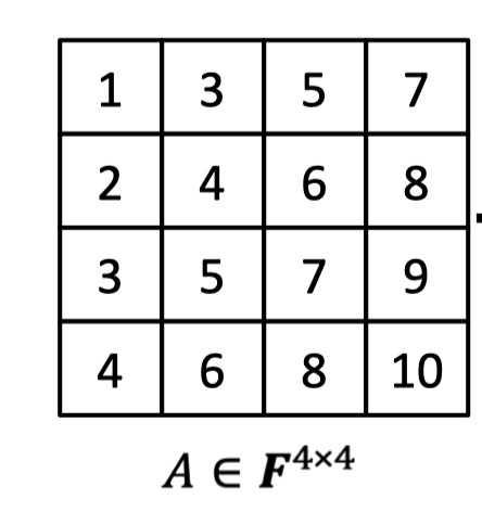
Note that the domain of function $A$ is $\{0,1\}^{2\log n}$, which has $2\log n$ variables as inputs. It make sense to extend function $A$ to its multilinear polynomial $\tilde{A}$ with domain $\mathbb{F}^{2\log n}$, each variable having degree at most 1.

Hence, we can define a polynomial $g(X,Y,Z)=\tilde{A}(X,Y)\tilde{A}(Y,Z),\tilde{A}(X,Z)$ that has $3\log n$ variables, each variable having degree at most 2.

Having defined the function $g$ with domain $\{0,1\}^{3\log n}$, the prover and the verifier simply apply the sum-check protocol to $g$ to compute:

$$ \sum_{(a,b,c)\in \{0,1\}^{3\log n}}g(a,b,c) $$

In summary, the design of the protocol is as follows.

Protocol:

• View $A$ as a function mapping $\{0,1\}^{\log n}\times \{0,1\}^{\log n}$ to $\mathbb{F}$.
• Extend $A$ to obtain its multilinear extension denoted by $\tilde{A}$.
• Define the polynomial $g(X,Y,Z)=\tilde{A}(X,Y)\tilde{A}(Y,Z),\tilde{A}(X,Z)$.
• Apply the sum-check protocol to $g$ to compute $\sum_{(a,b,c)\in \{0,1\}^{3\log n}}g(a,b,c)$.

Costs:

Note that $g$ has $3\log n$ variables and it has degree at most 2 in each variable.

• Total communication is $O(\log n)$.
• Verifier runtime is $O(n^2)$.
  • The total communication is logarithmic.
  • Hence, the verifier runtime is dominated by evaluating $g$ at one point $g(r_1,r_2,r_3)=\tilde{A}(r_1,r_2)\tilde{A}(r_2,r_3)\tilde{A}(r_1,r_3)$, which amounts to evaluating $\tilde{A}$ at three points.
  • The matrix $A$ gives the lists of all $n^2$ evaluations of the multilinear extension $\tilde{A}:\{0,1\}^{2\log n}\rightarrow \mathbb{F}$. As described above, the **verifier** can in linear time evaluate the multilinear extension function at any desired point in $\mathbb{F}^{2\log n}$.
  • Note that the verifier runtime is linear to the size of the input/matrix, that’s $O(n^2)$.
• Prover runtime is $O(n^3)$.
  • The prover’s runtime is clearly at most $O(n^5)$ since there are $3\log n$ rounds and $g$ can be evaluated at any point in $O(n^2)$ time.
  • But more sophisticated algorithm insights can bring the prover runtime down to $O(n^3)$. We recommend reader to refer to Chapter 4 and Chapter 5 in Thaler

A SNARK for circuit-satisfiability

We can apply the sum-check protocol to design SNARKs for circuit satisfiability.

Given an arithmetic circuit $C$ over $\mathbb{F}$ of size $S$ and output $y$. $P$ claims to know a $w$ such that $C(x,w)=y$.

For simplicity, let’s take $x$ to be the empty input.

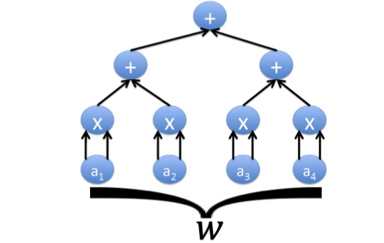
A transcript $T$ for $C$ is an assignment of a value to every gate as follows.

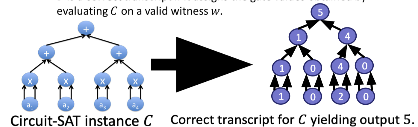
$T$ is a correct transcript if it assigns the gate values obtained by evaluating $C$ on a valid witness $w$.

The main idea is to assign each gate in $C$ a $(\log S)$-bit label and view such a transcript as a function with domain $\{0,1\}^{\log S}$ mapping to $\mathbb{F}$.

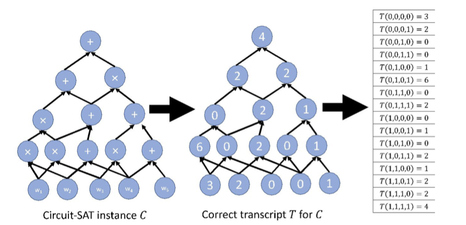
Hence, $P$’s first message is a $(\log S)$-variate polynomial $h$ claimed to extend a correct transcript $T$, which means

$$ h(x)=T(x) \text{ }\forall x\in \{0,1 \}^{\log S} $$

As usual, $T$ is defined over the hypercube $\{0,1\}^{\log S}$ and $h$ is multilinear extension of $T$ with domain $\mathbb{F}^{\log S}$.

$V$ can check this claim by evaluating all $S$ evaluations on $h$.

Like the sum-check protocol, suppose the verifier is only able to learn a few evaluations of $h$ rather than $S$ points.

Intuition of extension function

Before describing the design details, let’s dig the intuition for why we use the extension polynomial $h$ of the transcript $T$ for $P$ to send.

Intuitively, we think $h$ as a distance-amplified encoding of the transcript $T$.

The domain of $T$ is $\{0,1\}^{\log S}$. The domain of $h$ is $\mathbb{F}^{\log S}$, which is vastly bigger.

By Schwart-Zippel lemma, if two transcripts disagree at even a single gate value, their extension polynomial $h,h’$ disagree at almost all points in $\mathbb{F}^{\log S}$. Specifically, a $1-\log (S)/|\mathbb{F}|$ fraction.

The distance-amplifying nature of the encoding will enable $V$ to detect even a single “inconsistency” in the entire transcript.

As a result, it kind of blows up the tiny difference in transcripts by the extension polynomials into easily detectable difference so that it can be detectable even by the verifier that is only allowed to evaluate the extension polynomials at a single point or a handful points.

Two-step plan of attack

The original claim the prover makes is that the $(\log S)$-variate polynomial $h$ extends the correct transcript.

In order to offload work of the verifier and apply the sum-check protocol, the prover instead claims a related $(3\log S)$-variate polynomial $g_h=0$ at every single boolean input, i.e. $h$ extends a correct transcript $T$ ↔ $g_h(a,b,c)=0$ $\forall (a,b,c)\in \{0,1\}^{3\log S}$.

Moreover, to evaluate $g_h(r)$ at any input $r$, suffices to evaluate $h$ at only 3 inputs. Specifically, the first step is as follows.

Step 1: Given any $(\log S)$-variate polynomial $h$, identify a related $(3\log S)$-variate polynomial $g_h(a,b,c)$ via

$$ \widetilde{add}(a,b,c)\cdot (h(a)-(h(b)+h(c))+\widetilde{mult}(a,b,c)\cdot (h(a)-h(b)\cdot h(c)) $$

1. $\widetilde{add},\widetilde{mult}$ are multilinear extension called wiring predicates of the circuit. $\widetilde{add}(a,b,c)$ splits out 1 iff $a$ is assigned to an addition gate and its two input neighbors are $b$ and $c$. Likewise, $\widetilde{mult}(a,b,c)$ splits out 1 iff $a$ is assigned to the product of values assigned to $b$ and $c$.
2. $g_h(a,b,c)=h(a)-(h(b)+h(c))$ if $a$ is the label of a gate that computes the sum of gates $b$ and $c$.
3. $g_h(a,b,c)=h(a)-(h(b)\cdot h(c))$ if $a$ is the label of a gate that computes the product of gates $b$ and $c$.
4. $g_h(a,b,c)=0$ otherwise.

---

Then we need to design an interactive proof to check that $g_h(a,b,c)=0 \text{ } \forall (a,b,c)\in \{0,1\}^{3\log S}$ in which $V$ only needs to evaluate $g_h(r)$ at one random point $r\in \mathbb{F}^{3\log S}$.

It is very different from the zero test.

Using zero test, we are able to check $g_h=0$ for any input in $\mathbb{F}^{3\log S}$ by evaluating a random point $r$, but now we need to check $g_h=0$ over a hypercube $\{0,1\}^{3\log S}$.

Imagine for a moment that $g_h$ were a univariate polynomial $g_h(X)$.

And rather than needing to check that $g_h$ vanishes over input set $\{0,1\}^{3\log S}$, we need to check that $g_h$ vanishes over some set $H\subseteq \mathbb{F}$.

We can design the polynomial IOP based on following fact.

Fact:

$g_h(x)=0$ for all $x\in H$ ↔ $g_h$ is divisible by $Z_H(x)=\prod_{a\in H}(x-a)$.

We call $Z_H$ the vanishing polynomial for $H$.

The polynomial IOP works as follows. More details can be referred to the next Lecture.

Polynomial IOP:

1. $P$ sends a polynomial $q$ such that $g_h(X)=q(X)\cdot Z_H(X)$.
2. $V$ checks this by picking a random $r\in \mathbb{F}$ and checking that $g_h(r)=q(r)\cdot Z_H(r)$.

However, it dosen’t work when $g_h$ is not a univariate polynomial. Moreover, having $P$ find and send the quotient polynomial is expensive for high-degree polynomial.

In the final SNARK, this would mean applying polynomial commitment to additional polynomials. This is what Marlin, Plonk and Groth16 do. In the next lecture, we will elaborate on the Plonk.

---

Instead, the solution is to use the sum-check protocol.

Concretely speaking, the sum-check protocol is able to handle multivariate polynomials and dosen’s require $P$ to send additional large polynomials.

For simplicity, imagine working over the integers instead of $\mathbb{F}$.

The general idea is as follows.

(Note that it is not a full version of solution.)

Step2: General Idea of IP

• $V$ checks this by running sum-check protocol with $P$ to compute:

  $$ \sum_{a,b,c\in \{0,1\}^{\log S}}g_h(a,b,c)^2 $$
  • If all terms in the sum are 0, the sum is 0.
  • If working over the integers, any non-zero term in the sum will cause the sum to be strictly positive.

• At end of sum-check protocol, $V$ needs to evaluate $g_h(r_1, r_2, r_3)$.

  • Suffices to evaluate $h(r_1),h(r_2),h(r_3)$.
  • Outside of these evaluations, $V$ runs in time $O(\log S)$ with $3\log S$ rounds.
  • $P$ performs $O(S)$ field operations given a witness $w$.