「Cryptography-ZKP」: Lec5-The Plonk SNARK

In this series, I will learn Zero Knowledge Proofs (ZKP) on this MOOC, lectured by Dan Boneh, Shafi Goldwasser, Dawn Song, Justin Thaler and Yupeng Zhang.
Any corrections and advice are welcome. ^ - ^

Topics:

• Preprocessing SNARK
• KZG Poly-Commit Scheme
• Proving Properties of committed polys
  • ZeroTest
  • Product Check
  • Permutation Check
  • Prescribed Permutation Check
• Plonk IOP for General Circuits

What is SNARK?

Before proceeding to today’s topic, let’s review what is SNARK.

Note that this part is well explained in Lecture 2.

preprocessing NARK

NARK is Non-interactive ARgument of Knowledge.

Given a public arithmetic circuit $C(x,w)\rightarrow \mathbb{F}$ where $x$ is the public statement in $\mathbb{F}^n$ and $w$ is the secret witness in $\mathbb{F}^m$, a preprocessing (setup) algorithm

$$
S(C)\rightarrow \text{ public parameters } (pp,vp)
$$

takes a description of the circuit as inputs, and outputs public parameters $(pp,vp)$ for prover and verifier.

NARK works as follows.

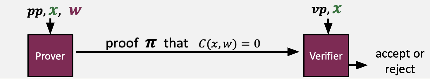
A preprocessing NARK is a triple of algorithms $(S,P,V)$.

• $S(C)\rightarrow$ public parameters $(pp,vp)$ for prover and verifier.
• $P(pp,x,w)\rightarrow$ proof $\pi$.
• $V(vp,x,\pi)\rightarrow$ accept or reject.

Note that all algorithms and the adversary have access to a random oracle.

The informal requirements of NARK are completeness and adaptively knowledge soundness.

Completeness means that an honest prover always convinces the verifier to accept the answer, i.e.

$$ \forall x,w: C(x,w)=0 \text{ then } \operatorname{Pr}[V(vp,x,P(pp,x,w))=\text{accept}]=1 $$

Adaptively knowledge soundness means that if the verifier accepts the proof, then the prover must know a witness such that $C(x,w)=0$. In other words, there exists an extractor $E$ that can extract a valid $w$ from $P$.

Zero-knowledge suggests that $(C,pp,vp,x,\pi)$ reveals nothing new about $w$. Note that the privacy requirement, i.e. zero knowledge, in NARK is optional. So there is a trivial NARK in which the prover just sends $w$ as proof and the verifier just rerun the circuit and check if $C(x,w)=0$.

SNARK: a Succinct ARgument of Knowledge

SNARK is a NARK (complete and knowledge sound) that is succinct.

zk-SNARK is a SNARK that is also zero knowledge, meaning that the SNARK proof reveals nothing about the witness.

A preprocessing SNARK is a triple of algorithms $(S,P,V)$.

• $S(C)\rightarrow$ public parameters $(pp,vp)$ for prover and verifier.
• $P(pp,x,w)\rightarrow$ short proof $\pi$; $\text{len}(\pi)=\text{sublinear}(|w|)$.
• $V(vp,x,\pi)\rightarrow$ fast to verify; $\text{time}(V)=O_\lambda(|x|,\text{sublinear}(|C|))$.

SNARK requires the length of proof to be sublinear in the length of the witness, and the verify runtime to be linear in the statement and sublinear in the size of the circuit.

Being linear in the statement $x$ means that the verifier at least read the statements.

Furthermore, a strongly succinct preprocessing NARK is not only sublinear but logarithmic in the size of the circuit.

• $S(C)\rightarrow$ public parameters $(pp,vp)$ for prover and verifier.
• $P(pp,x,w)\rightarrow$ short proof $\pi$; $\text{len}(\pi)=O_\lambda(\log(|C|))$.
• $V(vp,x,\pi)\rightarrow$ fast to verify; $\text{time}(V)=O_\lambda(|x|,\log (|C|))$.

Note that the verifier runtime is logarithmic in the size of the circuit, which implies that the verifier even does not know what the underlying circuit is.

An insight is that the verifier parameter $vp$ is the short “summary” of the circuit so the verifier is able to verify the evaluations of the circuit at an arbitrary input $x$.

That’s the reason why we need the preprocessing or setup.

It is worth noting that the trivial SNARK is not a SNARK.

Types of preprocessing Setup

The setup for a circuit $C$ is an algorithm $S(C;r)\rightarrow \text{ public parameters}(pp,vp)$, which takes the circuit and random bits as inputs and generates public parameters for the prover and the verifier.

The types of setup are more detailed.

• trusted setup per circuit: random $r$ must be kept secret from the prover.
  • $S(C;r)$
• trusted but universal (updatable) setup: secret $r$ is independent of $C$.
  • $S=(S_{init},S_{index})$
  • $S_{init}(\lambda;r)\rightarrow gp$: onetime setup, secret $r$
  • $S_{index}(gp,C)\rightarrow (pp,vp)$: deterministic algorithm
• transparent setup: does not use secret data
  • $S(C)$

In the trusted setup, random $r$ must be kept secret from the prover, meaning that it has to be run for every circuit.

Once the prover learns $r$, it allows the prover to prove false statements. In practice, $r$ will be destroyed so that nobody can ever know $r$. Sometimes, it is called the trusted setup ceremony.

In the trusted but universal setup, it splits the setup into two parts. $S_{init}$ is a one-time setup that does not take the circuit as input and generates global parameters $gp$. Note that $r$ is required to be secret as well.

Then $S_{index}$ is a deterministic algorithm executed for every circuit so it takes the circuit and $gp$ as inputs and generates public parameters for the prover and the verifier.

In the transparent setup, $S(C)$ does not use secret data.

General Paradigm for Building SNARK

The general paradigm for building SNARK is made up of two steps.

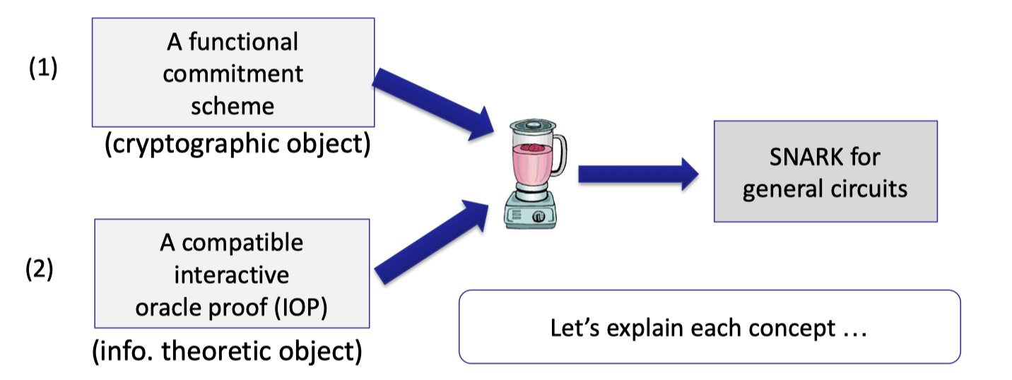
One is the functional commitment scheme, which is a cryptographic object that depends on some assumptions.

The other is the compatible interactive oracle proof (IOP). IOP is an information-theoretic object, which provides unconditional security without any assumptions.

To be precise, they are not separate steps.

For example, using poly-IOP, we can boost polynomial functional commitment for $\mathbb{F}_p^{(\le d)}[X]$ to build SNARK for any circuit $C$ where $|C|<d$.

Polynomial Commitments

Review the polynomial commitments introduced in the last lecture.

Prover commits to a univariate polynomial $f(X)$ in $\mathbb{F}_p^{(\le d)}[X]$ where the variable $X$ has degree at most $d$.

Later the verifier can request to know the evaluation of this polynomial at a specific point.

In other words, for public $u,v\in \mathbb{F}_p$, the prover can convince the verifier that the committed polynomial satisfies

$$
f(u)=v \text{ and deg}(f)\le d
$$

Note that the verifier has the upper bound of the degree $d$, the commitment received from the prover, and $u,v$.

In SNARK, the evaluation proof size and verifier time should be logarithmic in the degree, i.e. $O_\lambda(\log d)$.

Equality Test Protocol

Recall the observation that if $p,q$ are univariate polynomials of degree at most $d$, then $\operatorname{Pr}_{r\overset{\$}\leftarrow \mathbb{F}}[p(r)=q(r)]\le d/p$.

If $f(r)=g(r)$ for a random $r \overset{\$}\leftarrow \mathbb{F}_p$, then $f=g$ w.h.p. Having the polynomial commitments, we can construct the equality test protocol as follows.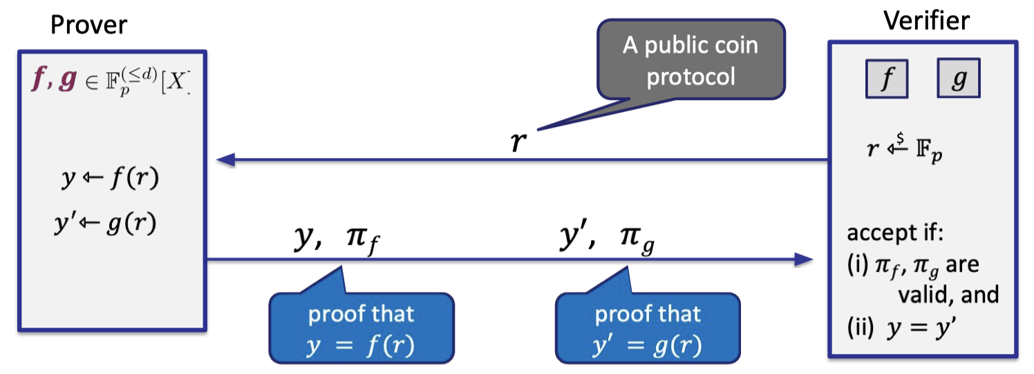

1. Prover has committed to two polynomial $f,g$, so verifier has two commitments depicted in two boxes.
2. Verifier samples a random coin $r$ in $\mathbb{F}_p$ and sends to prover.
   Hence, it is a public coin.
3. Prover sends the evaluations $y,y’$ and proof that $y=f(r)$ and $y’=g(r)$.
4. Verifier accepts if $y=y’$ and the proof is valid.

Fiat-Shamir Transform

Note that the equality teat protocol is interactive but the verifier just sends coins to prover.

A solution to making it a SNARK (non-interactive) is the Fiat-Shamir transform, which can render a public-coin interactive protocol non-interactive.

Let $H:M\rightarrow R$ be a cryptographic hash function.

The main idea is having prover generates verifier’s random bits on its own using $H$, i.e. $r\leftarrow H(x)$.

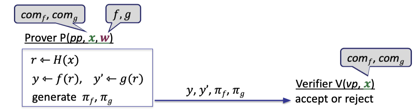
Prover and verifier can compute $r\leftarrow H(x)$, making it non-interactive.

The completeness is evident and one has to prove knowledge soundness.

Thm via Fiat-Shamir Transform:

This is a SNARK if ( i ) $d/p$ is negligible where $f,g\in \mathbb{F}_p^{(\le d)}[X]$, and ( ii ) $H$ is modeled as a random oracle.

In practice, we use SHA256 as $H$.

The succinctness holds by a succinct poly commitment scheme.

Note that it is not zk since verifier learns the value of $f(r),g(r)$ that he didn’t know before.

---

In this blog, we’ll introduce a specific polynomial commitment scheme — KZG’10 with a trusted setup.

KZG requires a trusted but universal setup that generates global parameters once, then it can commit to an arbitrary polynomial of bounded degree $d$.

$\mathcal{F}$-IOP

Having the functional commitments, we can build SNARKs for some circuits, e.g. zero test, equality test.

But with $\mathcal{F}$-IOP, we can boost functional commitment to build SNARK for any circuit $C(x,w)$.

Hence, $\mathcal{F}$-IOP is a proof system that proves $\exist w:C(x,w)=0$ as follows.

• Setup: The setup algorithm outputs public parameters for prover and verifier where $vp$ contains a number of oracles for functions in $\mathcal{F}$.
  Verifier can ask the oracle for evaluations at some points.
  The oracles will be replaced to functional commitment schemes in SNARKs.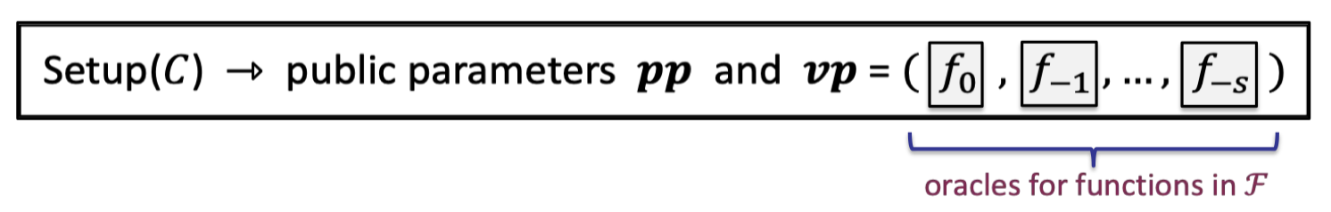

  

• IP proving $C(x,w)=0$: In each round, prover sends an oracle for a function $f_i$ which later on the verifier can evaluate at any point of his choice.
  Likewise, the oracles will be compiled to the commitment scheme when instantiating actual SNARKs.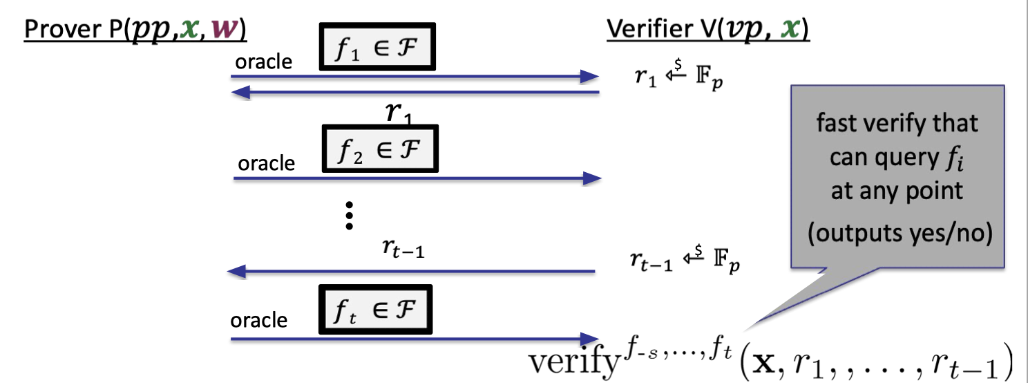

  

Properties:

• Complete: if $\exist w:C(x,w)=0$ then $\operatorname{Pr}[\text{verifier accepts}]=1$.
• (Unconditional) knowledge sound (as an IOP): extractor is given $(x,f_1, r_1, \dots, r_{t-1},f_t)$ and outputs $w$.
  Note that the given functions are in clear since the functional commitments are SNARKs so the extractor can extract the functions from the commitments.
• Optional: zero knowledge for a zk-SNARK

KZG Poly-Commit Scheme

Let’s introduce today’s highlight, KZG polynomial commitment scheme [Kate-Zaverucha-Goldberg’2010].

KZG: A Binding PSC

Fixed a group $\mathbb{G}={0,G,2\cdot G, 3\cdot G,\dots, (p-1)\cdot G}$ of order $p$.

Commitment

It requires a trusted but universal setup.

• $\text{setup}(1^\lambda)\rightarrow gp$
  • Sample random $\tau\in \mathbb{F}_p$
  • $gp=(H_0=G,H_1=\tau\cdot G, H_2=\tau^2\cdot G, \dots, H_d=\tau^d \cdot G)\in \mathbb{G}^{d+1}$.
  • delete $\tau$!!
• $\text{commit}(gp,f)\rightarrow \text{com}_f$ where $\text{com}_f=f(\tau)\cdot G \in \mathbb{G}$
  • $f$ as prover parameter
  • $\text{com}_f$ as verifier parameter

The setup generates global parameters $gp$ in which the random $\tau$ used must be destroyed.

Then prover can use $gp$ to generate the commitment for any specific polynomial $f\in \mathbb{F}_p^{(\le d)}[X]$.

It is worth noting the prover can compute $f(\tau)\cdot G$ without knowing $\tau$.

It can be evaluated by $gp$:

$$
\begin{aligned}f(X)& =f_0+f_1X+\dots+f_d X^d \ \text{com}_f &= f_0 \cdot H_0 +\dots f_d\cdot H_d \ &=f_0\cdot G + f_1\tau \cdot G +f_2 \tau^2\cdot G +\cdots \ &= f(\tau)\cdot G\end{aligned}
$$

where $f_0,\dots, f_d$ are coefficients of the polynomial.

This is a binding commitment but not hiding since it reveals $f(\tau)\cdot G$.

Evaluation

After committing to $f$, verifier can request for evaluations at a specific point.

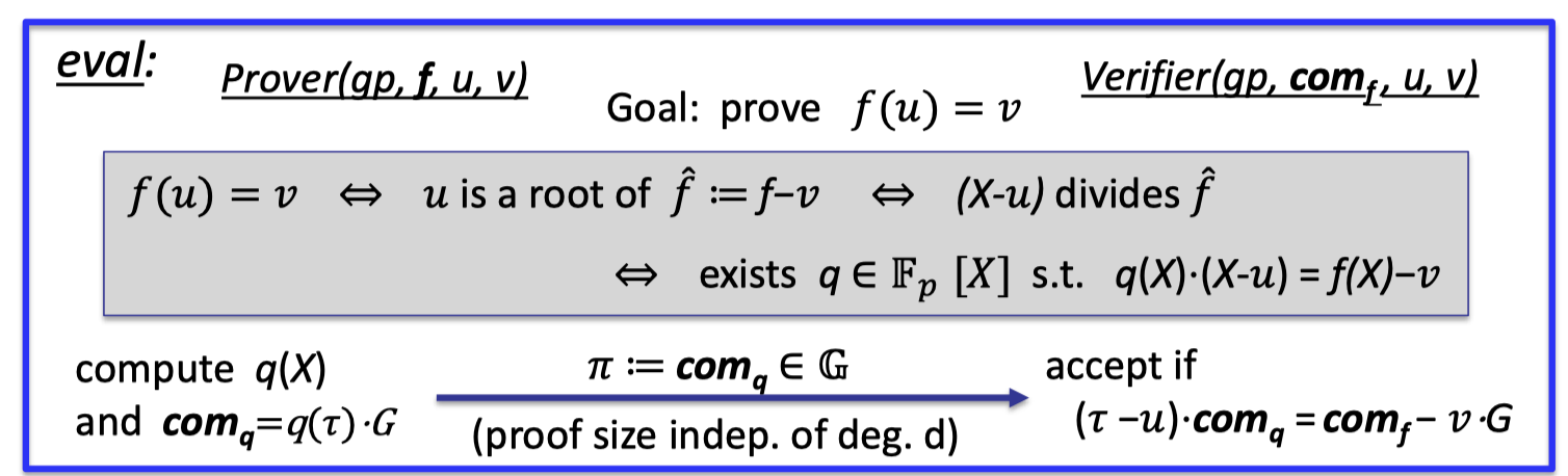
For public $u,v\in \mathbb{F}_p$, the prover can convince the verifier that the committed polynomial satisfies $f(u)=v$.

The proof hinges on some cute algebraic properties:

• $f(u)=v$ iff
• $u$ is a root of $\hat{f}=f-v$ iff
• $(X-u)$ divides $\hat{f}$ iff
• exists $q\in \mathbb{F}_p[X]$ s.t. $q(X)\cdot (X-u)=f(X)-v$

As a result, we can construct an equality test on two polynomials to verify the original claim $f(u)=v$.

The whole idea is depicted as follows.

Eval:

• Prover
  • compute the quotient polynomial $q(X)$ and $\text{com}_q=q(\tau)\cdot G$ as the commitment.
  • send the proof $\pi:=\text{com}_q\in \mathbb{G}$
  • Note that the proof is just one group element, which is const size better than logarithmic in $d$.
• Verifier
  • accept if $(\tau-u)\cdot \text{com}_q=\text{com}_f -v\cdot G$
  • The equality test for $(X-u)q(X)\cdot G=(f(X)-v)\cdot G$ can be checked by the random $\tau$.

It is worth noticing that $\tau$ is secret.

But verifier can use a “pairing” to do the above computation with only $H_0,H_1$ from $gp$, which is a fast computation for verifier.

As for the prover, computing the quotient is indeed an expensive computation for large $d$.

Generalizations

There are two ways to generalize KZG.

• [PST’13] Can use KZG to commit to $k$-variate polynomials.
• Batch proofs: Can commit to $n$ polynomials and provide a batch proof for multiple evaluations.
  • suppose verifier has commitments $\text{com}_{f_1},\dots, \text{com}_{f_n}$
  • prover wants to prove $f_i(u_{i,j})=v_{i,j}$ for $i\in [n],j\in[m]$
  • → batch proof $\pi$ is only one group element !

Properties: linear time commitment

One wonderful property of KZG is the prover’s runtime for commitment is linear in the degree $d$.

There are two ways to represent a polynomial $f(X)$ in $\mathbb{F}_p^{(\le d)}[X]$:

• Coefficient representation:
  $f(X)=f_0+f_1X+\dots +f_d X^d$.
  • computing $\text{com}_f=f_0\cdot H_0 +\dots +f_d\cdot H_d$ takes linear time in $d$.
• Point-value representation:
  $((a_0,f(a_0)),\dots,(a_d,f(a_d))$
  • computing $\text{com}_f$ naively: construct coefficients $(f_0,f_1,\dots, f_d)$ takes time $O(d\log d)$ using Number Theoretic Transform (NTT).

Using the point-value representation, the naive way of constructing coefficients takes time $O(d\log d)$ yet we want it linear in $d$.

A better way to compute the commitment with point-value representation is the Lagrange interpolation.

$$ f(\tau)=\sum_{i=0}^d \lambda_i (\tau)\cdot f(a_i) \\ \text{where } \lambda_i(\tau)=\frac{\prod_{j=0,j\ne i}^d (\tau -a_j)}{\prod _{j=0,j\ne i}^{d}(a_i-a_j)}\in \mathbb{F}_p $$

One can transform $gp$ into Lagrange form $\hat{gp}$ by a linear map, not involving any secrets so that anyone can fulfill this transformation.

$$ \hat{gp}=(\hat{H}_0=\lambda_0(\tau)\cdot G,\hat{H}_1=\lambda_1(\tau)\cdot G,\dots, \hat{H_d}=\lambda_d(\tau)\cdot G) $$

Now, prover can in linear time computes the commitment from the point-value representation as follows.

$$ \text{com}_f=f(\tau)\cdot G=f(a_0)\cdot \hat{H}_0+\dots +f(a_d)\cdot \hat{H}_d $$

To sum up, prover can compute the commitment in linear time from the coefficient representation or the point-value representation.

Multi-point Proof Generation

Let $\Omega\subseteq \mathbb{F}_p$ and $|\Omega|=d$.

Consider such a case in which prover has some $f(X)$ in $\mathbb{F}_p^{(\le d)}[X]$ and needs evaluation proofs $\pi_a\in G$ for all $a\in \Omega$.

When it comes to generate evaluation proofs for multi-points, prover naively takes time $O(d^2)$ for $d$ proofs, each takes time $O(d)$.

Feist-Khovratovich (FK2020) algorithm optimize to

• time $O(d\log d)$ if $\Omega$ is a multiplicative subgroup
• time $O(d\log^2 d)$ otherwise.

The Dory polynomial commitment

The difficulties with KZG lies in two parts

One has to require trusted setup for $gp$, and $gp$ size is linear in $d$.

Dory (eprint/2020/1274) is proposed to get over the trusted setup.

• transparent setup: no secret randomness in the setup
• $\text{com}_f$ is a single group element (independent of degree $d$ )
• eval proof size for $f\in \mathbb{F}_p^{(\le d)}[X]$ is $O(\log d)$ group elements.
  Note the eval proof size is constant size in original KZG.
• eval verify time is $O(\log d)$
  Note the eval verify time is constant.
• prover time is $O(d)$

Applications: vector commitment

Polynomial Commitment Scheme (PCS) have many applications.

One is to perform a drop-in replacement for Merkle trees.

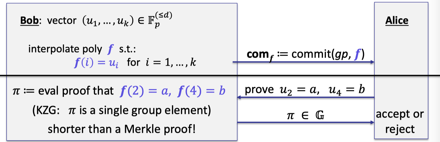
The idea is to view the vector $(u_1,\dots, u_k)\in \mathbb{F}_p^{(\le d)}$ as a function $f$ such that $f(i)=u_i$ for $i=1,\dots, k$, then prover can commits to this polynomial.

Instead of proving the revealed entry is consistent with the committed vector, prover can generate evaluation proof that $f(2)=a,f(4)=b$ as depicted follows.

The proof $\pi$ is a single group element (using batch proof) that is shorter than a Merkle proof.

Proving properties of committed polynomials

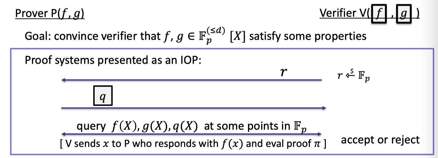
Having PCS, not only verifier can query evaluations of a committed polynomial, but prover can convince verifier that the committed polynomials $f,g$ satisfy some properties, e.g. equality test.

It can be summed up in the following process.

• Start: Prover has functions $f,g$ in clear and verifier has the corresponding commitments via PCS.
• Verifier samples a random $r\in \mathbb{F}_p$.
• Prover computes a related polynomial $q$ and commits to it.
• Verifier can query $f,g,q$ at point $x$ and accept if valid.
  Note that when we say verifier query a committed polynomial $f(x)$, it means verifier sends $x$ to prover who responds with $f(x)$ and eval proof $\pi$. (described in here[link])

Polynomial Equality Testing with KZG

As described above, we can construct equality test for two committed polynomials.

But for KZG, $f=g$ if and only if $\text{com}_f=\text{com}_g$, resulting that verifier can tell if $f=g$ on its own.

But prover is needed to test equality of computed polynomials.

For example, verifier has four individual commitments to $f,g_1,g_2,g_3$ where all four are in $\mathbb{F}_p^{(\le d)}[X]$ to test $f=g_1g_2g_3$.

Then verifier queries all four polynomials at a random point $r\overset{$}\leftarrow \mathbb{F}_p$ and tests equality.

It is complete and sound assuming $3d/p$ is negligible since $\text{deg}(g_1g_2g_3)\le 3d$.

Summary of Proof Gadgets for Univariates

In order to construct Poly-IOPs for an arbitrary circuit.

In this section, we’ll introduce some important proof gadgets for univariates.

Let $\Omega$ be some subset of $\mathbb{F}_p$ of size $k$.

Let $f\in \mathbb{F}_p^{(\le d)}[X]$ where $d\ge k$ and verifier has the commitment to $f$.

We can construct efficient Poly-IOPs for the following tasks.

• Zero Test: prove that $f$ is identically zero on $\Omega$.
• Sum Check: prove that $\sum_{a\in \Omega}f(a)=0$.
• Prod Check: prove that $\prod_{a\in \Omega}f(a)=1$.
  • → prove for rational functions that $\prod_{a\in \Omega}f(a)/g(a)=1$
• Permutation Check: prove that $g(\Omega)$ is the same as $f(\Omega)$, just permuted.
• Prescribed Permutation Check: prove that $g(\Omega)$ is the same as $f(\Omega)$, permuted by the prescribed $W$.

Vanishing Polynomial

Before staring, let’s introduce the vanishing polynomial.

Def: Vanishing Polynomial of $\Omega$:

The vanishing polynomial of $\Omega$ is

$$
Z_\Omega(X):=\prod_{a\in \Omega}(X-a)
$$

such that $\text{deg}(Z_\Omega)=k$.

By definition, the vanishing polynomial is a univariate polynomial to be $0$ everywhere on subset $\Omega$.

We can construct a cute vanishing polynomial by constructing a special subset $\Omega$.

Let $\omega\in \mathbb{F}_p$ be a primitive $k$-th root of unity so that $\omega ^k=1$.

If $\Omega=\{1,\omega, \omega^2, \dots, \omega^{k-1}\}\subseteq \mathbb{F}_p$ then $Z_\Omega(X)=X^k-1$.

Then for $r\in \mathbb{F}_p$, evaluating $Z_\Omega(r)$ takes $\le 2\log_2{k}$ field operations by repeated squaring algorithm.

It’s super fast.

In the following tasks, we fix $\Omega=\{1,\omega, \omega^2, \dots, \omega^{k-1}\}$.

ZeroTest on $\Omega$

In zero test, prove wants to convince verifier that $f$ is identically zero on $\Omega$.

We build zero test by the following lemma.

Lemma:

$f$ is zero on $\Omega$ if and only if $f(X)$ is divisible by $Z_{\Omega}(X)$.

The IOP of zero test is depicted as follows.

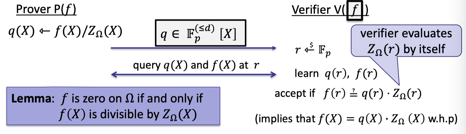
1. Prover computes the quotient polynomial $q(X)=f(X)/Z_{\Omega}(X)$ and commits to this polynomial.

   Note that with KZG prover can only commits to a polynomial in $\mathbb{F}_p^{(\le d)}$ rather than a rational functions.

2. Verifier samples a random $r\in \mathbb{F}_p$.

3. Verifier query $q(X)$ and $f(X)$ at point $r$ to learn $q(r)$ and $f(r)$. And verifier evaluates $Z_\Omega(r)$ by itself.

4. Verifier accepts if $f(r)=q(r)\cdot Z_\Omega(r)$ since it implies $f(X)=q(X)\cdot Z_\Omega(X)$ w.h.p.

Theorem:

This protocol is complete and sound assuming $d/p$ is negligible.

Costs:

• Verifier time: $O(\log k)$ for evaluating $Z_\Omega(r)$ plus two poly queries (that can be batch into one)
• Prover time: dominated by the time to compute $q(X)$ and then commit to $q(X)$.

Product Check on $\Omega$

We omit the details of sum check and jump to the product check since they are nearly the same.

Product check is a useful gadget to construct the permutation check introduced later.

In product check, prover wants to convince verifier that the products of all evaluations over $\Omega$ equals to $1$, i.e.

$$
\prod_{a\in \Omega}f(a)=1
$$

We construct a degree-$k$ polynomial to prove it.

Set $t\in \mathbb{F}_p^{(\le k)}[X]$ to be the degree-$k$ polynomial such that

$$
\begin{aligned}t(1)&=f(1), \ t(\omega^s)&=\prod_{i=0}^s f(\omega^i) \text{ for }s=1,\dots, k \end{aligned}
$$

Note that a degree-$k$ polynomial can be uniquely specified by $k+1$ points.

Then $t(\omega^i)$ evaluates the prefix-products as follows.

• $t(\omega)=f(1)\cdot f(\omega)$,
• $t(\omega^2)=f(1)\cdot f(\omega)\cdot f(\omega^2)$
• … …
• $t(\omega^{k-1})=\prod_{a\in \Omega}f(a)=1$

We can represent prefix-product in a iterative way:

$$
t(\omega\cdot x)=t(x)\cdot f(\omega \cdot x) \text{ for all }x\in \Omega
$$

As a result, we can do the product check by the following lemma, which can be proved with the evaluation proof and a zero test.

Lemma: If

( i ) $t(\omega^{k-1})=1$ and

( ii ) $t(\omega\cdot x)-t(x)\cdot f(\omega\cdot x)=0$ for all $x\in \Omega$

then $\prod_{a\in \Omega}f(a)=1$.

The IOP for product check is depicted as follows.

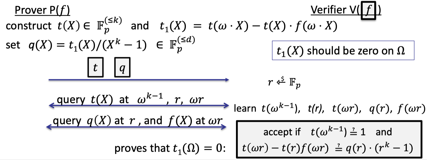
We can split it two parts:

• Evaluation proof to prove $t(\omega^{k-1})=1$
  • Prover construct $t(X)\in \mathbb{F}_p^{(\le k)}$ and commits to it.
  • Verifier queries $t(X)$ at $\omega^{k-1}$.
  • check1: Verifier checks that if $t(\omega^{k-1})=1$.
  • proof size: one commit, one evaluation.

Let $t_1(X)=t(\omega\cdot X)-t(X)\cdot f(\omega\cdot X)$.

• Zero test to prove $t_1$ is zero on $\Omega$.
  Recall the lemma that $t_1$ is zero on $\Omega$ iff $Z_{\Omega}(X)$ divides $t_1(X)$.
  • Prover computes the quotient polynomial $q(X)=t_1(X)/(X^{k}-1)\in \mathbb{F}_p^{(\le d)}$ and commits to it.
  • Verifier samples a random $r\in \mathbb{F}_p$ and need to learn $t_1(r)$ and $q(r)$.
    • Verifier queries $q(X)$ at $r$.
    • Verifier queries $t(X)$ at $\omega r$, and $r$.
    • Verifier u $f(X)$ at $\omega r$.
  • Verifier computes $r^{k}-1$ in time $O(\log k)$.
  • check2: Verifier checks if $t(\omega\cdot r)-t(\omega)\cdot f(\omega\cdot r)=q(r)\cdot (r^k-1)$.
  • proof size: one commit, four evaluations.

Note that it is a public-coin interactive protocol that can be rendered non-interactive via Fiat-Shamir Transform.

To sum up, the proof size is made up of two commits and five evaluations (can be batched into a single group element).

Theorem:

This protocol is complete and sound assuming $2d/p$ is negligible.

( $t(X)\cdot f(\omega\cdot X)$ has degree at most $2d$ ).

It takes verifier $O(\log k)$ time to compute $r^{k-1}-1$.

It takes prover $O(k\log k)$ time to compute $t(X)$ and $q(X)$ using the naive way that constructs the coefficients from the point-value representation.

---

Likewise, it works to prove the products on rational functions:

$$
\prod_{a\in \Omega}(f/g)(a)=1
$$

We construct a similar degree-$k$ polynomial to prove it.

Set $t\in \mathbb{F}_p^{(\le k)}[X]$ to be the degree-$k$ polynomial such that

$$
\begin{aligned}t(1)&=f(1)/g(1), \ t(\omega^s)&=\prod_{i=0}^s f(\omega^i)/g(\omega^i) \text{ for }s=1,\dots, k \end{aligned}
$$

We write the prefix-product in an iterative way:

$$
t(\omega\cdot x)=t(x)\cdot \frac{f(\omega \cdot x)}{g(\omega\cdot x)} \text{ for all }x\in \Omega
$$

Then we can prove the following two parts to fulfill the product check.

Lemma: If

( i ) $t(\omega^{k-1})=1$ and

( ii ) $t(\omega\cdot x)\cdot g(\omega \cdot x)-t(x)\cdot f(\omega\cdot x)=0$ for all $x\in \Omega$

then $\prod_{a\in \Omega}f(a)/g(a)=1$.

Note that the proof size is two commits and six evaluations.

Theorem:

This protocol is complete and sound assuming $2d/p$ is negligible.

Compared to the original prod-check, the one extra evaluation comes from the query to $g(X)$ at $\omega\cdot r$.

Permutation Check

Let $f,g$ be polynomials in $\mathbb{F}_p^{(\le d)}[X]$.

Verifier has commitments to $f$ and $g$.

In permutation check, that goal is that prover wants to prove that $(f(1),f(\omega),f(\omega^2),\dots, f(\omega^{k-1})\in \mathbb{F}_p^k$ is a permutation of $(g(1),g(\omega),g(\omega^2),\dots, g(\omega^{k-1}))\in \mathbb{F}_p^k$.

It means to prove that $g(\Omega)$ is the same as $f(\Omega)$, just permuted.

The main idea is to construct auxiliary polynomials that have the evaluations as its root.

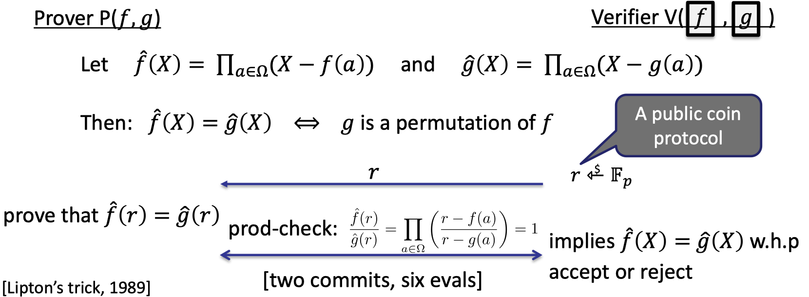
Let $\hat{f}(X)=\prod_{a\in \Omega}(X-f(a))$ and $\hat{g}(X)=\prod_{a\in \Omega}(X-g(a))$.

Then $\hat{f}(X)=\hat{g}(X)$ if and only if $g$ is a permutation of $f$ on $\Omega$.

The thing to notice is that prover cannot just commits to $\hat{f}$ and $\hat{g}$, then verifier checks if $\hat{f}(r)=\hat{g}(r)$.

Because there is a missed proof that $\hat{f}$ is honestly constructed by the committed $f$.

Instead, prover is needed to prove $\hat{f}(r)=\hat{g}(r)$ by performing a product check on a rational function $\frac{r-f(X)}{r-g(X)}$.

The IOP for permutation check is depicted as follows.

Let’s elaborate on the details.

• Start: Prover has functions $f,g$ in clear and verifier has commitments to $f,g$.

1. Verifier samples a random $r$.

2. Prover constructs $\hat{f}$ using the evaluations of $f$, so is $\hat{g}$.

3. Then prover wants to prove $\hat{f}(r)=\hat{g}(r)$.

   1. It can be transformed to prove $\frac{\hat{f}(r)}{\hat{g}(r)}=1$ where $r$ is fixed.

   2. They can perform prod-check to prove

      $$
      \frac{\hat{f}(r)}{\hat{g}(r)}=\prod_{a\in \Omega}\left(\frac{r-f(a)}{r-g(a)}\right)=1
      $$

      where the rational function is defined as $\frac{r-f(X)}{r-g(X)}$ on $\Omega$.

• Proof size: two commits and six evaluations, same as prod-check on rational functions.

It’s a public-coin protocol that can be rendered non-interactive.

Theorem:

This protocol is complete and sound assuming $2d/p$ is negligible.

Prescribed Permutation Check

Let’s look into an embellished permutation check where the permutation is prescribed by a specific permutation $W$.

We say $W:\Omega\rightarrow \Omega$ is a permutation of $\Omega$ if $\forall i\in [k]$: $W(\omega^i)=\omega^j$ is bijection.

A bijection means one-to-one correspondence.

A bijection function is injective and surjective.

Let $f,g$ be polynomials in $\mathbb{F}_p^{(\le d)}[X]$.

Verifier has three individual commitments to $f, g,$ and $W$.

In prescribed permutation check, the goal of prover is to prove that $f(y)=g(W(y))$ for all $y\in \Omega$.

In other works, it proves that $g(\Omega)$ is the same as $f(\Omega)$, permuted by the prescribed $W$.

---

At first sight, we try to use a zero-test to prove $f(y)-g(W(y))=0$ on $\Omega$.

But the problem is the polynomial $f(y)-g(W(y))$ has degree $k^2$ since $g(W(y))$ is a composition of $f$ and $W$.

Then prover would need to manipulate polynomials of degree $k^2$, resulting a quadratic time prover !!

Yet we want a linear time prover.

---

Let’s reduce this to a prod-check on a polynomial of degree $2k$.

Observation:

If $(W(a),f(a))_{a\in \Omega}$ is a permutation of $(a, g(a))_{a\in \Omega}$,

then $f(y)=g(W(y))$ for all $y\in \Omega$.

By the definition of permutation, for $a\in \Omega$, there exists a $a’\in \Omega$ $W(a’)=a$ and $f(a’)=g(a)$ hold. Then we have $f(a’)=g(W(a’))$.

The following example illustrates the proof.

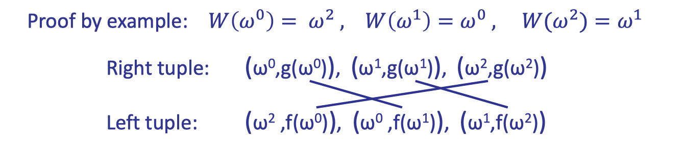
Likewise, we construct auxiliary polynomials that have the evaluations as its root yet the evaluations are listed in form of the tuple.

The intuition is to encode the tuple to a variable, then use a similar way to construct a bivariate polynomial that has the variables as its root.

Hence, the tuple is encoded as variables $Y\cdot W(a)+f(a)$ and $Y\cdot a+g(a)$, respectively.

And the bivariate polynomials of total degree $k$ is constructed as follows.

$$ \begin{cases} \hat{f}(X,Y)&= \prod _{a\in \Omega}(X-Y\cdot W(a)-f(a)) \\ \hat{g}(X,Y) &= \prod_{a\in \Omega}(X-Y\cdot a -g(a))\end{cases} $$

The following lemma shows the correctness.

Lemma:

$\hat{f}(X,Y)=\hat{g}(X,Y)$ if and only if $(W(a),f(a))_{a\in \Omega}$ is a permutation of $(a,g(a))_{a\in \Omega}$.

To prove, use the fact that $\mathbb{F}_p[X,Y]$ is a unique factorization domain. Yet I’m not familiar with this fact.

The complete protocol is depicted as follows, which composes a prod-check on the rational function $\frac{r-s\cdot W(X)-f(X)}{r-s\cdot X-g(X)}$ where $r,s$ are fixed and randomly chosen by the verifier.

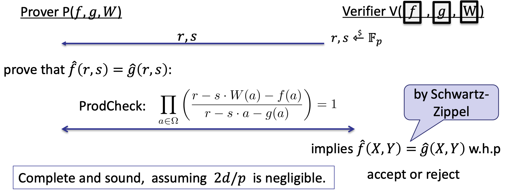
Theorem:

This protocol is complete and sound assuming $2d/p$ is negligible.

The PLONK IOP for General Circuits

PLONK

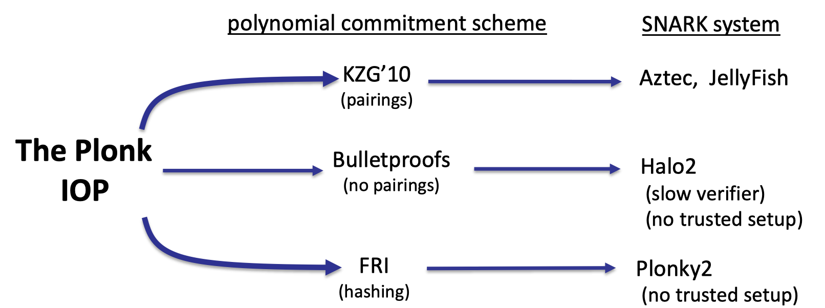
Finally, let’s introduce PLONK IOP, a widely used proof system in practice.

It is a poly-IOP for a general circuit $C(x,w)$.

We can think the PLONK IOP as an abstract IOP that can be combined with different polynomial commitment schemes to construct actual SNARK system.

Step1: compile circuit to a computation trace

The first step is to compile a general circuit to a computation trace that can be encoded by a polynomial.

Considering a general circuit $(x_1+x_2)(x_2+w_1)$ with two public inputs and one witness input, we can write the computation trace into a table as follows. This compilation is also called arithmetization.

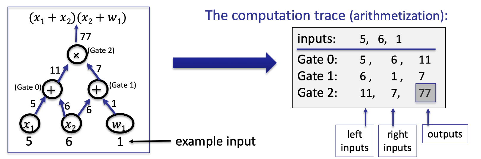
The example is illustrated as above.

Let $|C|$ denote the total # of gates in $C$.

Let $|I|=|I_x|+|I_w|$ denote the # inputs to $C$.

Let $d=3|C|+|I|$ and $\Omega=\{1,\omega, \omega^2, \dots, \omega^{d-1}\}$ where $\omega\in \mathbb{F}_p$ is the primitive $k$-th root of unity so that $\omega ^d=1$.

In the above example, $|C|=3$, $|I|=3$, and $d=12$.

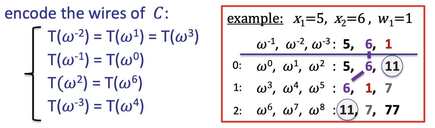
The plan is prover can interpolates a polynomial $T\in \mathbb{F}_p^{(\le d)}[X]$ that encodes the entire trace.

1. $T$ encodes all inputs: $T(\omega^{-j})=\text{input }\# j \text{ for } j=1,\dots, |I|$.
2. $T$ encodes all wires: $\forall l=0,\dots, |C|-1$:
   For each gate labeled by $l$,
   1. $T(\omega^{3l})$: left input to gate $\#l$
   2. $T(\omega^{3l+1})$: right input to gate $\#l$
   3. $T(\omega^{3l+2})$: output to gate $\#l$

In our example, prover interpolates $T(X)$ of degree 11 such that:

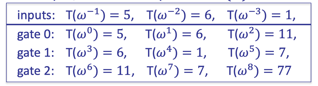
Note that prover can use FFT / NTT to compute the coefficients of $T$ in time $O(d\log d)$.

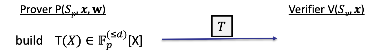
Step2: proving validity of $T$

Then prover commits to the polynomial $T$ encoded by the computation trace, and needs to prove that $T$ is a correct computation trace.

Proving Validity of :

1. $T$ encodes the correct inputs.
2. Every gate is evaluated correctly.
3. The wiring is implemented correctly.
4. The output of last gates is 0.
   (In our example, the output is 77)

Proving (4) is easy that only proves $T(\omega^{3|C|-1})=0$.

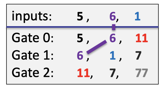
The wiring constraints contains that the second input $6$ is connected with the left wire of the gate 0 and the right wire of the gate 1 as depicted as follows.

(1) $T$ encodes the correct input

Note that the statement $x$ is public.

Both prover and verifier interpolate a polynomial $v(X)\in \mathbb{F}_p^{(\le |I_x|)}[X]$ that encodes the $x$-inputs to the circuit:

$$ \text{for }j=1,\dots, |I_x|: v(\omega^{-j})=\text{input }\# j $$

In our example, $v(\omega^{-1})=5,v(\omega^{-2})=6$, hence $v$ is linear.

Note that constructing $v(X)$ takes time proportional to the size of input $x$ so that verifier has time to do this.

Let $\Omega_{\text{inp}}=\{\omega^{-1},\omega^{-2},\dots, \omega^{-|I_x|}\}\subseteq \Omega$ that contains the points encoding the inputs.

Prover proves (1) by using ZeroTest on $\Omega_{\text{inp}}$ to prove that

$$
T(y)-v(y)=0 ; \forall y\in \Omega_{\text{inp}}
$$

Note that verifier can construct $v(X)$ explicitly so verifier only query $T(X)$ at randomly chosen $r$.

(2) every gate is evaluated correctly

Suppose that the circuit only composes the additional gates and multiplication gates.

The idea of differentiating is to encode gate types using a selector polynomial $S(X)$.

Define $S(X)\in\mathbb{F}_p^{(\le d)}[X]$ such that $\forall l=0, \dots, |C|-1$:

$$ \begin{cases}S(\omega^{3l})&= 1 \text{ if gate }\# l \text{ is an addition gate} \\ S(w^{3l})&=0\text{ if gate }\# l \text{ is an multiplication gate}\end{cases} $$

In our example, the selector polynomial is interpolated as follows.

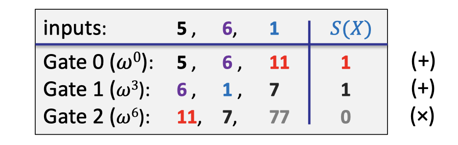
The selector polynomial will be committed in the preprocessing phase because it is a function of the circuit, which just encodes what the gates represent in the circuit.

With the selector polynomial, we can encode the addition gates and the multiplication gates into a single polynomial.

$$ \forall y\in \Omega_{\text{gates}}=\{1,\omega^3,\omega^6,\omega^9,\dots, \omega^{3(|C|-1)}\}: \\ S(y)\cdot [T(y) + T(\omega y)] + (1-S(y))\cdot T(y)\cdot T(\omega y)=T(\omega^2 y) $$

If the above equality holds, it means that all the addition gates and multiplication gates are evaluated correctly.

• $\#l$ is an **addition gate** → $S(y=\omega^{3l})=1$
  • Prove that the sum of the left input and right input equals to the output, i.e. $T(y)+T(\omega y)=T(\omega^2 y)$.
• $\#l$ is a **multiplication gate** → $S(y=\omega^{3l})=0$
  • Prove that the product of the left input and right input equals to the output, i.e. $T(y)\cdot T(\omega y)=T(\omega^2 y)$.

Then prover uses ZeroTest to prove that for $\forall y\in \Omega_{\text{gates}}$:

$$
S(y)\cdot [T(y) + T(\omega y)] + (1-S(y))\cdot T(y)\cdot T(\omega y)-T(\omega^2 y)=0
$$

(3) the wiring is correct

The last thing is to prove the wiring is correct.

First we construct the wiring constraints to encode the wires of $C$.

In our example, the(incomplete) wiring constraints are listed as follows. The first constraint means that the second input is connected to the right input of the gate 0 and the left input of the gate 1.

Then define a polynomial $W:\Omega\rightarrow \Omega$ that implements a rotation:

• $W(\omega^{-2},\omega^{1},\omega^3)=(\omega^{1},\omega^3,\omega^{-2})$
• $W(\omega^{-1},\omega^0)=(\omega^{0},\omega^{-1})$
• … …

The rotation means $W$ maps $\omega^{-2}$ → $\omega^{1}$, $w^1$ → $\omega^3$, and $\omega^3$→ $\omega^{-2}$.

It means the polynomial $T$ is invariant under this rotation.

Note that $W$ actually defines a prescribed permutation.

Finally, the following lemma tells us we can prove the wiring constraints using a prescribed permutation check.

Lemma:

$\forall y\in \Omega$: if $T(y)=T(W(y))$, then wire constraints are satisfied.

It’s a clever way of encoding all the wiring constraints.

Note that the polynomial $W$ doesn’t depend on the inputs so it represents an intrinsic property of the circuit itself, which can be committed in the setup.

Complete Plonk Poly-IOP

The complete Plonk poly-IOP (and SNARK) is depicted as follows.

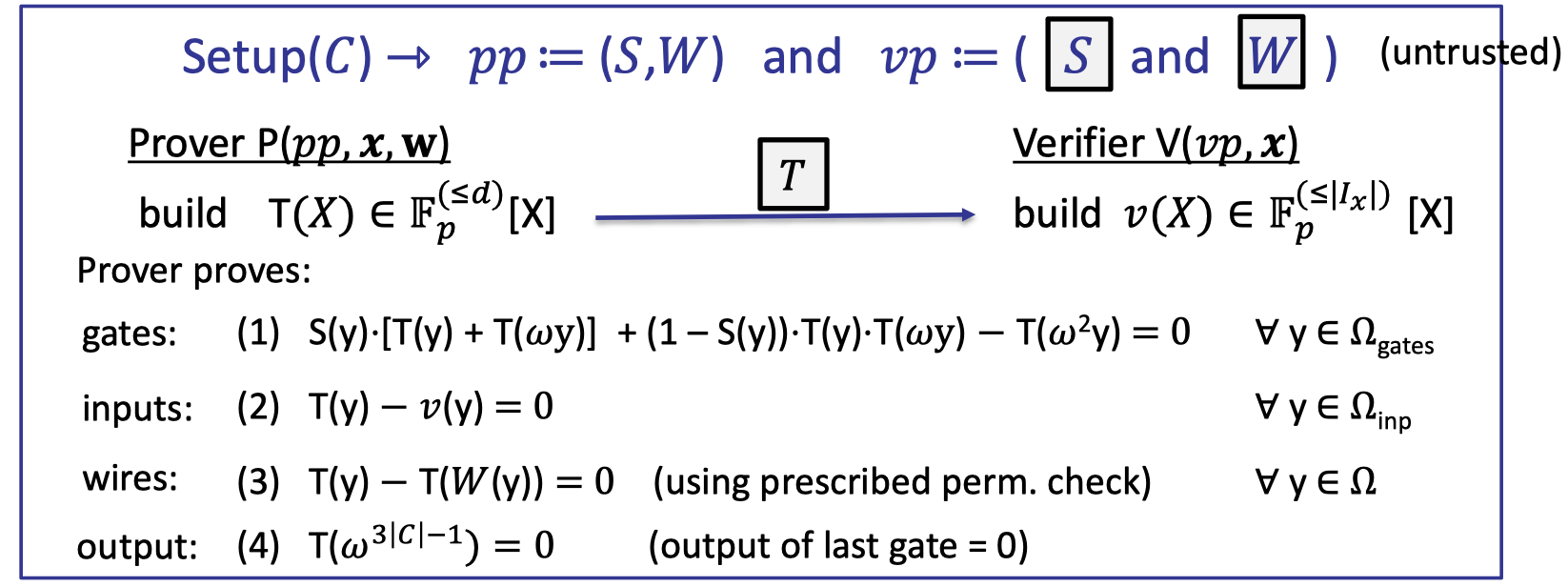
Let’s elaborate on the details.

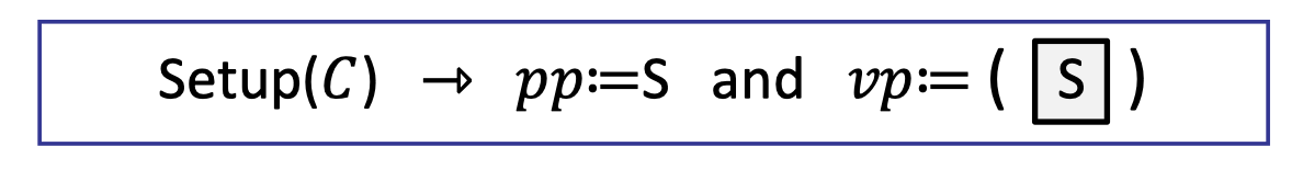
• The setup preprocesses the circuit $C$ and outputs the commitmens to the selector polynomial $S$ and the wiring polynomial $W$. It is untrusted that anyone can check these commitments were done correctly.
• Prover compiles the circuit to a computation trace, and encodes the entire trace into a polynomial $T(X)$.
• Verifier can construct $v(X)$ explicitly from the public inputs $x$.
• Then prover proves validity of $T$:
  • gates: evaluated correctly by ZeroTest
  • inputs: correct inputs by ZeroTest
  • wires: correct wirings by Prescribed Permutation Check
  • output: correct output by evaluation proof

Theorem:

The Plonk Poly-IOP is complete and knowledge sound, assuming $7|C|/p$ is negligible.

• $7|C|$ bounds the degree of the polynomial of $S\cdot T \cdot T$.
• constant proof size: a short proof with $O(1)$ commitments.
• fast verifier: runs in logarithmic time $O(\log |C|)$
• quasi-linear prover: $O(|C|\log |C|)$
• SNARK: rendered via Fiat-Shamir Transform

Note that the SNARK is not necessarily zk since the commitments are not zk and the openings are not as well.

But there are generic transformations that can efficiently convert any Poly-IOP into a zk Poly-IOP, rendering a zk-SNARK.

Extensions

Hyperplonk: linear prover

The main challenge in PLONK is the prover runs in quasi-linear time.

Hyperplonk replaces $\Omega$ with ${0,1}^t$ where $t=\log _2 |\Omega|$ to achieve a linear prover.

The polynomial $T$ is now a multilinear polynomial in $t$ variables, and the computation trace is encoded on the vertices of the $t$-dim hypercube.

ZeroTest is replaced by a multilinear SumCheck.

Recall that the prover time in SumCheck ([Lecture 4]) has a factor $2^t$, which is linear to $|C|$.

It turns out that all tools to build for proving facts about committed univariate polynomials can be generalized to work and prove properties of multilinear polynomials.

Plonkish Arithmetization

Another extension is about the arithmetization, including the custom gates and Plookup.

Having these extension allows to shrink the size of the computation traces, which speed up the prover runtime.

It supports custom gates other than addition gates and multiplication gates.

The plonkish computation trace can be illustrated as follows:

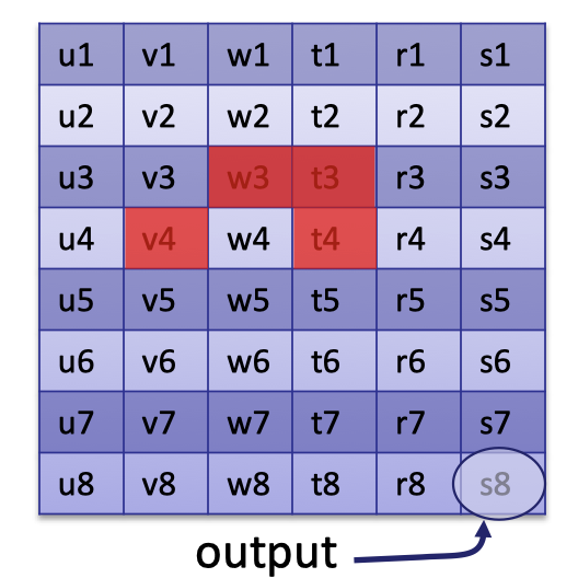
It is defined by a custom gate that computes $v_4+w_3\cdot t_3$ and outputs $t_4$.

Likewise, we can encode it into the following polynomial

$$
\forall y\in \Omega_{\text{gates}}: v(y\omega)+w(y)\cdot t(y)-t(y\omega)=0
$$

Prover uses a ZeroTest check to prove that the custom gate is evaluated correctly.

All such gate checks are included in the gate check by multiplying a selector polynomial.

Furthermore, Plookup can ensure some values in the computation trace are in pre-defined list.