「Cryptography-ZKP」: Lec6 Poly-commit based on Pairing and Discret-log

In this series, I will learn Zero Knowledge Proofs (ZKP) on this MOOC, lectured by Dan Boneh, Shafi Goldwasser, Dawn Song, Justin Thaler and Yupeng Zhang.
Any corrections and advice are welcome. ^ - ^

Topics:

• KZG poly-commit based on bilinear pairing
  • KZG scheme
  • Powers-of-tau Ceremony
  • Security Analysis
  • Knowledge of exponent assumption
  • Variants: multivariate; ZK; batch openings
• Bulletproofs poly-commit based on discrete logarithm

Before proceeding to today’s topic, let’s recall the common recipe for building an efficient SNARK.

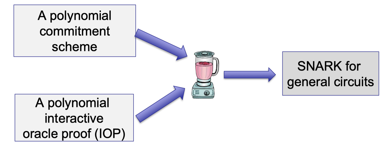
The common way of building SNARK is to combine a poly-IOP with a functional commitment scheme.

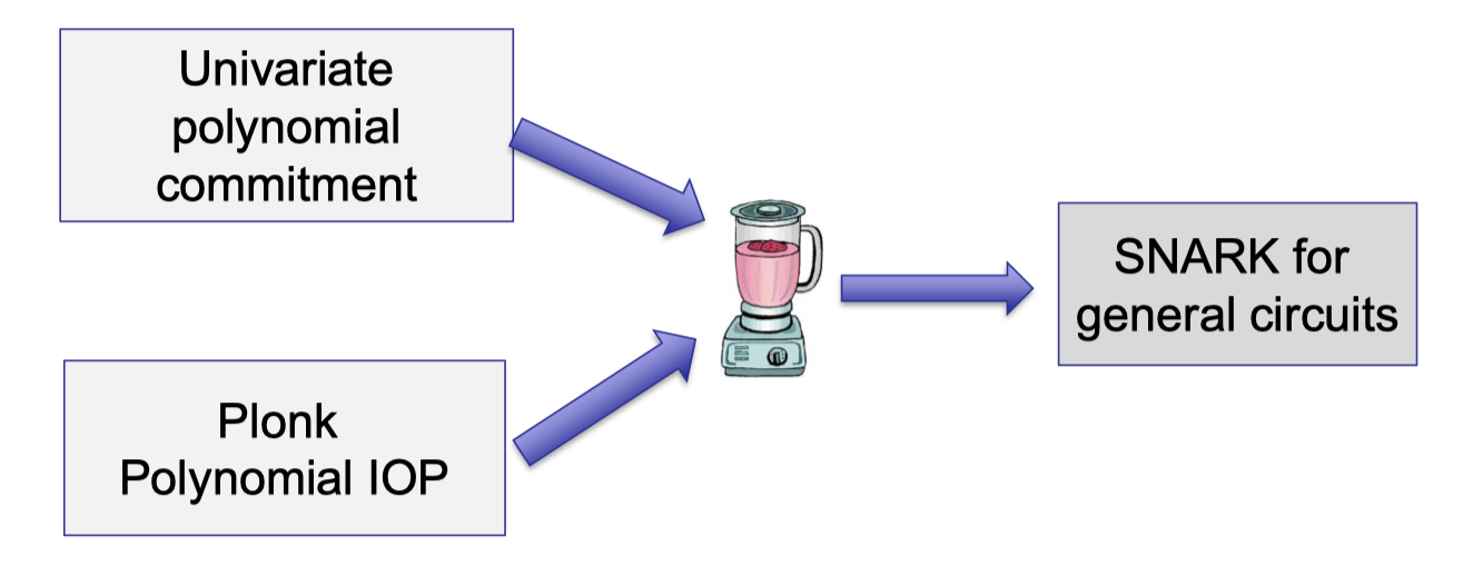
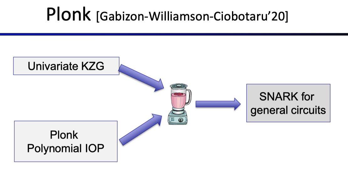
Lecture 4 uses Plonk (poly-IOP) combined with KZG (a univariate polynomial commitment) to build SNARK for general circuits.

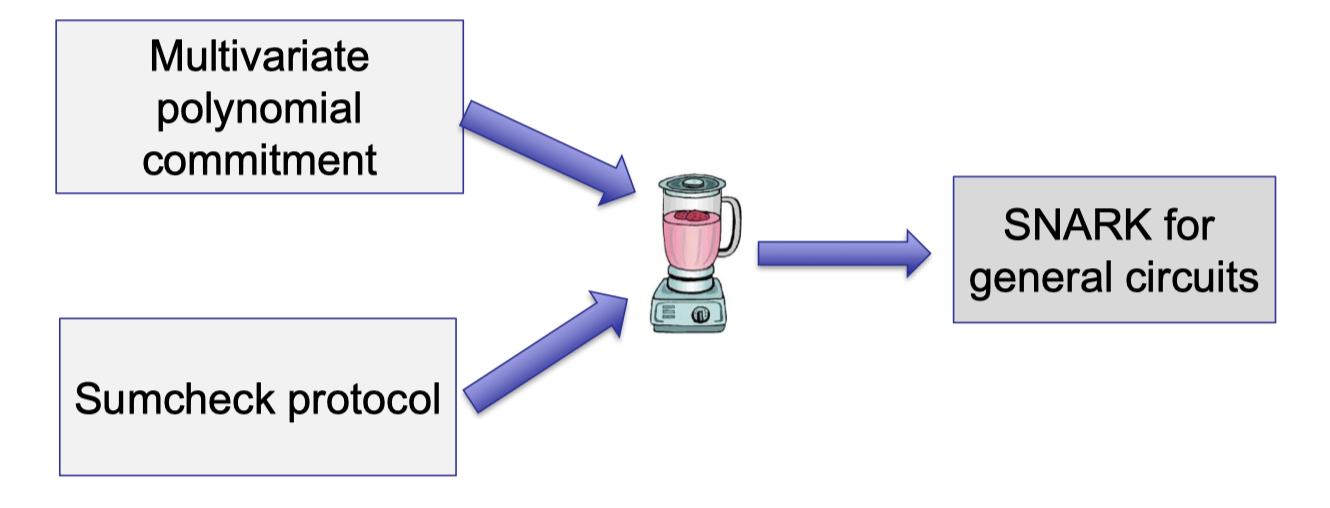
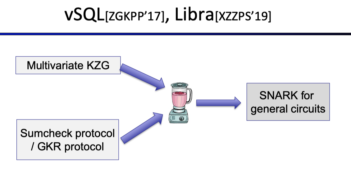
Lecture 3 uses Sumcheck protocol combined with a multivariate polynomial commitment to build SNARK.

In this lecture, we are going to introduce polynomial commitments based on bilinear pairing and discrete log.

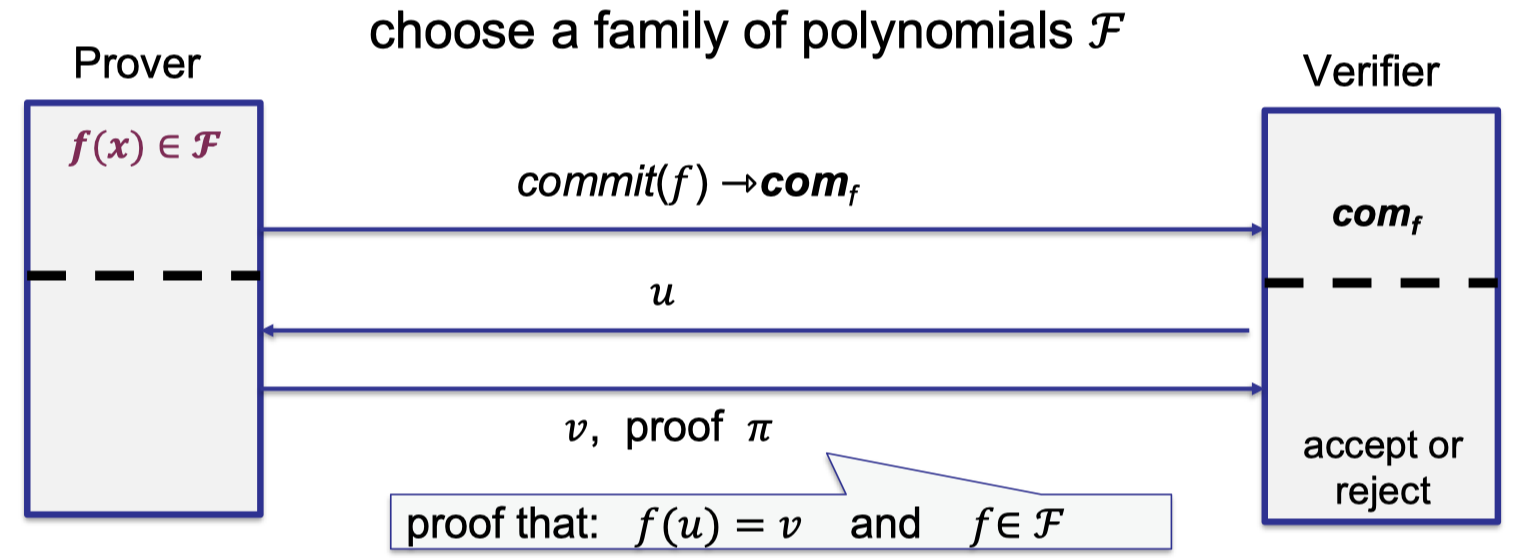
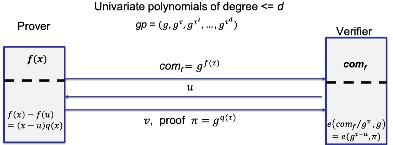
When building polynomial commitment schemes, we first choose a family of polynomial $\mathcal{F}$, then prover commits to a function $f(x)\in \mathcal{F}$.

Verifier receives $\text{com}_f$ as the commitment, then verifier is able to query $f$ at point $u$.

Finally, prover sends the evaluation $v$ and the proof $\pi$ that $f(u)=v$ and $f\in \mathcal{F}$, and verifier accepts if proof is valid.

The above procedure is depicted as follows.

For ease of use, we give a formal definition for polynomial commitment schemes (PCS).

It consists of four algorithms as follows.

• $\text{keygen}(\lambda, \mathcal{F})\rightarrow gp$
  In setup, this algorithm takes the family as inputs and outputs the global parameters used in the commitment and proof.
• $\text{commit}(gp,f)\rightarrow \text{com}_f$
  Prover calls this algorithm to commit to a function.
• $\text{eval}(gp,f,u)\rightarrow v,\pi$
  Prover calls this algorithm to compute the evaluation at the point $u$ and the corresponding proof.
• $\text{verify}(gp,\text{com}_f,u,v,\pi)\rightarrow \text{accept or reject}$
  Verifier calls this algorithm to check the validity of the proof and accept the answer if valid.

It is complete if an honest prover can convince the verifier to accept the answer.

It is sound if a verifier can catch a lying prover with high probability.

We compare the soundness and knowledge soundness in Lecture 3. To put it simply, soundness establishes the existence of the witness while knowledge soundness establishes that the prover necessarily knows the witness. As a result, knowledge soundness is stronger.

We give a formal definition of knowledge soundness.

Knowledge Sound:

For every poly. time adversary $A(A_0, A_1)$ such that

$$ \text{keygen}(\lambda,\mathcal{F})\rightarrow gp, A_0(gp)\rightarrow \text{com}_f, A_1(gp, u)\rightarrow v, \pi: \\ \operatorname{Pr}[V(vp, x,\pi)=\text{accept}]=1 $$

there is an efficient extractor $E$ (that uses $A$) such that

$$ \text{keygen}(\lambda,\mathcal{F})\rightarrow gp, A_0(gp)\rightarrow \text{com}_f, E(gp, \text{com}_f)\rightarrow f:\\ \operatorname{Pr}[f(u)=v \text{ and } f(x)\in \mathcal{F}]> 1-\epsilon $$

where $\epsilon$ is negligible.

Background

Let’s quickly go through the basic conceptions in number theory, which is widely used in the following sections.

I refer readers to This Blog for a detailed description.

Group: A set $\mathbb{G}$ and an operation $*$

1. Closure: For all $a,b\in \mathbb{G}$, $a* b \in \mathbb{G}$
2. Associativity: For all $a,b,c\in \mathbb{G}$, $(a*b)*c =a*(b*c)$
3. Identity: There exists a unique element $e\in \mathbb{G}$ s.t. for every $a\in \mathbb{G}$, $e*a=a*e=a$.
4. Inverse: For each $a\in \mathbb{G}$, there exists $b\in \mathbb{G}$ s.t. $a*b=b*a=e$.

A simple example is the group that contains integers $\{\dots, -2,-1,0,1,2,\dots\}$ under addition operation $+$. The common Groups considered in Cryptography are the group that contains positive integers mod prime $p:\{1,2,\dots, p-1\}$ under multiplication operation $\times$ and the groups defined by elliptic curves.

Generator of a group:

An element $g$ that generates all elements in the group by taking all powers of $g$.

For example, $3$ is a generator of the group $\mathbb{Z}_7^*={1,2,3,4,5,6}$.

We can write every group element in the power of $3$.

$3^1=3;3^2=2;3^3=6;3^4=4;3^5=5;3^6=1 \mod 7$

Discrete-log

A group $\mathbb{G}$ has an alternative representation as the powers of the generator $g:\{g,g^2, g^3,\dots,g^{p-1}\}$.

Discrete logarithm problem:

Given $y\in \mathbb{G}$, find $x$ such that $g^x=y$.

The quantum computer can actually solve the discrete logarithm problem in polynomial time.

Discrete logarithm assumption:

Discrete-log problem is computationally hard.

Note that the DL assumption does not hold in all groups but it is believed to hold in certain groups.

Computational Diffie-Hellman assumption:

Given $\mathbb{G},g,g^x,g^y$, cannot compute $g^{xy}$.

It is worth noting that a stronger assumption means the underlying problem is easier.

Hence, the CDH assumption is a stronger assumption than the DL assumption since the CDH problem is reducible to the DL problem.

Bilinear Pairing

The bilinear pairing is defined over $(p,\mathbb{G},g,\mathbb{G}_T,e)$.

• $\mathbb{G}$: the base group of order $p$, a multiplicative cyclic group
• $\mathbb{G}_T$: the target group of order $p$, a multiplicative cyclic group
• $g$: the generator of $\mathbb{G}$
• $e:\mathbb{G}\times \mathbb{G} \rightarrow \mathbb{G}_T$, the pairing operation

The pairing possesses the following bilinear property:

$$ \forall P,Q\in \mathbb{G}: e(P^x,Q^y)=e(P,Q)^{xy} $$

The pairing takes two elements in the base group $\mathbb{G}$ as inputs, and outputs an element of the target group.

For example, $e(g^x,g^y)=e(g,g)^{xy}=e(g^{xy},g)$.

By the CDH assumption, we know computing $g^{xy}$ is hard given $g^x$ and $g^y$. It means that computing the product in the exponent is hard.

But with pairing, we can check that some element $h=g^{xy}$ without knowing $x$ and $y$.

Note that with pairing, we cannot break the CDH assumption with pairing.

It actually gives us a tool to verify the product relationship in the exponent rather than computing the product in the exponent.

A pairing example is the BLS signature proposed by Boneh, Lynn, and Shacham in 2001. [Bonth-Lynn-Shacham’2001]

• $\text{Keygen}(p,\mathbb{G},g, \mathbb{G}_T,e):$ private key $x$ and public key $g^x$.
• $\text{Sign}(sk,m)\rightarrow \sigma:H(m)^x$ where $H$ is a cryptographic hash that maps the message space to $\mathbb{G}$.
• $\text{Verify}(\sigma, m):e(H(m),g^x)=e(\sigma,g)$

The verification is to check the pairing equation.

The LHS is the pairing of the hash of the message and the public key. The verifier cannot compute $H(m)^x$ without knowing $x$.

The RHS is the pairing of the signature and the generator.

Security Analysis:

The correctness holds since the verifier will pass if the signer honestly computes $H(m)^x$.

The idea of proving soundness is by contradiction.

Assuming there is an adversary that can forge a signature to pass the verification, then we can break CDH assumption using this bilinear group.

For your information, not all groups in which DL is hard are believed to support efficient computable pairing, but some groups especially those defined by elliptic curves.

KZG based on Bilinear Pairing

Lecture 4 has introduced KZG polynomial commitment scheme [Kate-Zaverucha-Goldberg’2010] with the multiplication notation but omits the details of pairing.

In this section, we use the exponent notation and consider a bilinear group defined by $p, \mathbb{G},g,\mathbb{G}_T,e$ and the univariate polynomials $\mathcal{F}=\mathbb{F}_p^{(\le d)}[X]$ with degree $\le d$.

Note that the degree $d$ is public to the verifier.

KZG scheme

Let’s elaborate on the four algorithms one by one.

keygen $(\lambda, \mathcal{F})\rightarrow gp$ : compute the global parameters

• $\text{keygen}(\lambda, \mathcal{F})\rightarrow gp$
  • Sample random $\tau\in \mathbb{F}_p$
  • $gp=(g,g^\tau,g^{\tau^2},\dots, g^{\tau^d})$
  • delete $\tau$ !! (trusted setup)

Intuitively, it uses a group where DL assumption is hard so that no one can compute $\tau$.

It suffices to use $gp$ to commit and generate the proof for the prover, and to check the pairing equation for the verifier, without knowing the secret $\tau$.

Once the prover learns the secret $\tau$, the prover can generate fake proof to fool the verifier and break the security of the polynomial commitment scheme.

It is worth noting that the secret $\tau$ should be deleted so that it requires a trusted setup, which is the main drawback of KZG.

For some practical applications, it is actually hard to find a trusted party to run a trusted setup.

commit $(gp,f)\rightarrow \text{com}_f$

• $f(x)=f_0+f_1x+f_2x^2+\dots+f_d x^d$

• $gp=(g,g^\tau,g^{\tau^2},\dots, g^{\tau^d})$

• Compute the commitment using $gp$

  $$ \begin{aligned}\text{com}_f&=g^{f(\tau)} \\ &=g^{f_0+f_1\tau +f_2\tau^2+\dots+f_d \tau^d} \\ &=(g)^{f_0} \cdot (g^{\tau})^{f_1} \cdot (g^{\tau^2})^{f_2}\dots (g^{\tau^d})^{f_d} \end{aligned} $$ ​

eval $(gp,f,u)\rightarrow v,\pi$

• $f(x)-f(u)=(x-u)q(x)$ as $u$ is a root of $f(x)-f(u)$
• Compute $q(x)$ and $\pi=g^{q(\tau)}$ using $gp$

Note that the proof can be computed without accessing $\tau$ and the proof size is only one group element.

Finally, we are going to introduce the verification part, which is the highlight of KZG.

The equation that the verifier wants to check is $f(x)-f(u)=(x-u)q(x)$.

A naive idea is to verify the equation at the point $\tau$ in the exponent on the base $g$.

$$ g^{f(\tau)-f(u)}=g^{(\tau-u)q(\tau)} $$

Verify has received $\text{com}_f=g^{f(\tau)}$ as commitment to $f$, $\pi=g^{q(\tau)}$ as eval proof, and $v=f(u)$ as evaluation from an honest prover.

Verifier can compute $g^{(\tau-u)}$ and $g^{q(\tau)}$ using $gp$.

Unfortunately, under CDH assumption, the verifier cannot compute $g^{(\tau-u)q(\tau)}$, which is the product in the exponent.

The solution is pairing, which gives us a way to check the relation in the exponent of the equation instead of computing it.

verify $(gp,\text{com}_f,u,v,\pi)$

• Idea: check the equation at point $\tau$

• Challenge: only know $g^{\tau-u}$ and $g^{q(\tau)}$

• Solution: pairing!

• Pairing!

  $$ \begin{aligned}e(\text{com}_f/g^v,g)&=e(g^{\tau-u},\pi) \\ e(g,g)^{f(\tau)-f(u)}&=e(g,g)^{(\tau-u)q(\tau)}\end{aligned} $$ ​

With pairing, the verifier can check the equation at the point $u$ in the exponent.

The complete protocol is depicted as follows.

Properties of KZG

Let’s sum up the properties of KZG poly-commit.

Properties of KZG:

• Keygen: trusted setup!
• Commit: $O(d)$ group exponentiations, $O(1)$ commitment size.
• Eval: $O(d)$ group exponentiations where $q(x)$ can be computed efficiently in linear time!
  Note: The polynomial division algorithm with nearly linear time is referred to this Lecture.
• Proof size: $O(1)$, 1 group element.
• Verifier time: $O(1)$, 1 pairing.

Powers-of-tau Ceremony

The main drawback of KZG is the requirement of a trusted setup.

A way to relax the trusted setup is Ceremony which uses a distributed generation of $gp$ so that no one can reconstruct the trapdoor if at least one of the participants is honest and discards their secrets.

The main idea of distributed generation is using the product of secrets from all parties.

The first party generates global parameters $gp=(g^\tau,g^{\tau^2},\dots, g^{\tau^d})=(g_1,g_2,\dots, g_d)$.

Then the next party samples random $s$, and update

$$ \begin{aligned}gp' &=(g_1',g_2',\dots, g_d') \\ &=(g_1^s,g_2^{s^2},\dots, g_d^{s^d}) \\ &= (g^{\tau s},g^{(\tau s)^2},\dots, g^{(\tau s)^d})\end{aligned} $$

with secret $\tau\cdot s$.

It introduces a secret $s$ from updating /ma

Finally, if all parties are honest, then the above procedure can generate the global parameters with the product of secrets from all parties.

Meanwhile, it is required to check the correctness of $gp’$.

Correctness of :

(See [Nikolaenko-Ragsdale-Bonneau-Boneh’22])

1. The contributor knows $s$ s.t. $g_1’=(g_1)^s$.
   It can be verified by the $\Sigma$ protocol.
2. $gp’$ consists of consecutive powers $e(g_i’,g_1’)=e(g’_{i+1},g)$, and $g_1’\ne 1$.

Note that the check of $g_1’\ne 1$ guarantees that the next party cannot remove the product of the preceding secrets and change it to 0.

Security Analysis

The completeness of KZG is evident.

The soundness of KZG is based on the following assumption.

$q$-Strong Bilinear Diffie-Hellman ($q$-SBDH) assumption:

Given $(p,\mathbb{G},g,\mathbb{G}_T,e)$ and $(g,g^\tau,g^{\tau^2},\dots, g^{\tau^d})$, cannot compute $e(g,g)^{\frac{1}{\tau-u}}$ for any $u$.

There is an exposition [Tanaka-Saito] of reductions among the $q$-strong Diffie-Hellman problem and related problems.

The $q$-SBDH problem is reducible to the CDH problem, so $q$-SBDH is a strictly stronger assumption.

Proof of Soundness: (By Contradiction)

Assume for contradiction that an adversary returns a wrong answer $v^*\ne f(u)$ but the fake proof $\pi^*$ pass the verification.

Then we can break $q$-SBDH assumption, which arrives to a contradiction.

• $e(\text{com}_f/g^{v^*})=e(g^{\tau-u},\pi^*)$
  • The pairing equation of verification holds by assumption.
• $e(g^{f(\tau)-v^{*}},g)=e(g^{\tau-u},\pi^*)$

  • Knowledge of Exponent (KoE) assumption

    Later we are going to introduce the KoE assumption, which proves that the prover necessarily knows $f$ s.t. $\text{com}_f=g^{f(\tau)}$ rather than a random element.

  • Because a random element as the commitment cannot be written in $g^{f(\tau)}$ for some $f$.

  • By KoE assumption, it means the prover necessarily knows an explicit $f$ so prover can compute $f(u)$.

• Define $\delta=f(u)-v^*$, which is $\ne 0$ by assumption.

  • This is the key idea of the proof that decomposes $v^*$ to the correct answer $f(u)$ and $\delta$.
• $\Leftrightarrow e(g^{\color{red}{f(\tau)-f(u)+f(u)-v^*}},g)=e(g^{\tau-u},\pi ^*)$

• $\Leftrightarrow e(g^{\color{red}{(\tau-u)q(\tau)+\delta}},g)=e(g^{\tau-u},\pi ^*)$

• $\Leftrightarrow e(g,g)^{(\tau-u)q(\tau)+\delta}=e(g,\pi ^*)^{\tau-u}$

• Then we can extract the common factor $\tau-u$ and put them outside the pairing to achieve our goal of computing$e(g,g)^{\frac{1}{\tau-u}}$.

• $\Leftrightarrow e(g,g)^{\delta}=(e(g,\pi ^*)/e(g,g)^{q(\tau)})^{\tau-u}$

• $\Leftrightarrow e(g,g)^{\frac{\delta}{\tau -u}}=e(g,\pi^*)/e(g^{q(\tau)},g)$

  • which breaks $q$-SBDH assumption.

Then we are going to prove knowledge soundness by the knowledge of exponent assumption.

Knowledge of Exponent assumption

In the above security proof, we assume that the prover necessarily knows $f$ such that $\text{com}_f=g^{f(\tau)}$ rather than a random element.

We make use of the Knowledge of Exponent (KoE) assumption to refine KZG protocol, achieving knowledge soundness.

I excerpt the following descriptions from [Bellare-Palacio’04] to intuitively introduce the knowledge of exponent assumption.

Let $q$ be a prime such that $2q+1$ is also prime (safe prime), and let $g$ be a generator of the order $q$ subgroup of $Z_{2q+1}^*$.

Suppose we are given input $q,g,g^a$ and want to output a pair $(C,Y)$ such that $Y=C^a$.

One way to do this is to pick some $c\in \mathbb{Z}_q$, let $C=g^c$, and let $Y=(g^a)^c$.

Intuitively, it can be viewed as saying that this is the “only” way to produce such a pair.

The assumption captures this by saying that any adversary outputting such a pair must “know” an exponent $c$ such that $g^c=C$.

The formalization asks that there be an “extractor” that can return $c$.

Knowledge of Exponent assumption :

For any adversary $A$ that takes input $q,g,g^a$ and returns $(C,Y)$ with $Y=C^a$, there exists an “extractor” $\bar{A}$, which given the same inputs as $A$ returns $c$ such that $g^c=C$.

KZG with Knowledge Soundness

Having this assumption, we can refine the KZG protocol.

The goal is to prove that prover necessarily “knows” an exponent $f(\tau)$ such that $\text{com}_f=g^{f(\tau)}$.

We’d like to ask the prover to generate such a pair $g^{f(\tau)}$ and $g^{\alpha f(\tau)}$ given “ $gp$ and $(gp)^{\alpha}$”.

The sketch of design is as follows.

Sketch:

• $gp=(g,g^\tau,g^{\tau^2},\dots, g^{\tau^d})$
• Sample random $\alpha$, compute $g^\alpha,g^{\alpha \tau},g^{\alpha \tau^2},\dots, g^{\alpha \tau^d}$
• $\text{com}_f=g^{f(\tau)}$ and $\text{com}’_f=g^{\alpha f(\tau)}$.
• If $e(\text{com}_f,g^\alpha)=e(\text{com}_f’,g)$, there exists an extractor $E$ that extracts $f$ s.t. $\text{com}_f=g^{f(\tau)}$.

Let’s elaborate on the details.

In addition to the original global parameters $gp$, we need to sample random $\alpha$ and compute $(gp)^\alpha:\{g^\alpha, g^{\alpha \tau}, g^{\alpha \tau^2},\dots, g^{\alpha\tau^d}\}$, which is raising each element of the original $gp$ to random $\alpha$.

Note that the random $\alpha$ is secret as $\tau$.

The prover commits to $f$ by computing such a pair, $\text{com}_f=g^{f(\tau)}$ and $\text{com}_f’=g^{\alpha f(\tau)}$.

Finally, the verifier can check the relation of these two commitments in the exponent by pairing.

If the pairing equation $e(\text{com}_f,g^\alpha)=e(\text{com}_f’,g)$ holds, by KoE assumption, there exists an extractor $E$ that extracts $f$ such that $\text{com}_f=g^{f(\tau)}$.

Here is the KZG scheme with knowledge soundness.

KZG with Knowledge Soundness:

• $\text{Keygen}$: $gp$ includes both $g,g^\tau,g^{\tau^2},\dots, g^{\tau^d}$ and $g^\alpha,g^{\alpha\tau},g^{\alpha\tau^2},\dots, g^{\alpha\tau^d}$ where $\tau$ and $r$ are both secret and required to be deleted. (trusted setup)
• $\text{Commit}$: $\text{com}_f=g^{f(\tau)}$ and $\text{com}_f’=g^{\alpha f(\tau)}$.
• $\text{Verify}$: additionally checks $e(\text{com}_f,g^\alpha)=e(\text{com}_f’,g)$.

The idea of proving knowledge soundness is to extract $f$ in the first step by the KoE assumption.

But it brings an overhead that the prove size is two group elements and the verifier time involves two pairing equations.

Generic Group Model (GGM) [Shoup’97, Maurer’05] can replace the KoE assumption and reduce the commitment size in KZG.

Informally speaking, the adversary is only given an oracle to compute the group operation. E.g., given $g,g^\tau,g^{\tau^2},\dots, g^{\tau^d}$, the adversary can only compute their linear combinations.

As a result, the adversary cannot sample a random element that happens to be the power of another group element.

See book “A Graduate Course in Applied Cryptography” by Dan Boneh and Victor Shoup, section 16.3 for more details.

Variants of KZG

Multivariate poly-commit

Reference: [Papamanthou-Shi-Tamassia’13]

KZG can be generalized to the multivariate polynomial commitment.

The key idea is the following equation:

$$ f(x_1,\dots, x_k)-f(u_1,\dots,u_k)=\sum_{i=1}^k (x_i-u_i) q_i(\vec{x}) $$

where $q(\vec{x})$ is a multivariate polynomial.

• Keygen: sample $\tau_1,\tau_2,\dots, \tau_k$, each representing one variable, and compute $gp$ as $g$ raised to all possible monomials of $\tau_1,\tau_2,\dots, \tau_k$.
  e.g. $2^k$ monomials for multilinear polynomials.
• Commit: $\text{com}=g^{f(\tau_1,\tau_2,\dots, \tau_k)}$
• Eval: compute $\pi_i=g^{q_i(\vec{\tau})}$.
  Note that the proof consists of multiple elements.
• Verify: $e(\text{com}_f/g^v,g)=\prod_{i=1}^ke(g^{\tau_i-u_i},\pi_i)$

Let $N\le 2^k$ denote the total size of the polynomial.

The proof size and verifier time are $O(\log N)$.

Achieving zero-knowledge

Reference: [ZGKPP’2018]

We say a poly-commit scheme is ZK if there is a simulator without knowing the polynomial can simulate the view of the verifier.

The plain KZG is not ZK. E.g. the commit algorithm $\text{com}_f=g^{f(\tau)}$ is deterministic.

The solution to achieve zero-knowledge is masking the commitment and proof with randomizers.

• Commit: $\text{com}_f=g^{f(\tau)+r\eta}$
• Eval: the main idea is to check whether a polynomial with randomizers is of a certain form.
  • bivariate polynomial with randomizer: $\begin{aligned} f(x)+ry-f(u) =(x-u)(q(x)+r’y)+y(r-r’(x-u))\end{aligned}$
  • proof: $\pi=g^{q(\tau)+r’\eta},g^{r-r’(\tau-u)}$

Let’s elaborate on the details.

First look at the commitment $\text{com}_f=g^{f(\tau)+r\eta}$.

The commitment to $f$ is randomized by $r$ randomly chosen by the prover.

Note that $\eta$ is another secret sampled in the trusted setup so $g^\eta$ is included in the global parameters, which enables the prover to compute it.

With random $r$ in the commitment, the idea of evaluation is to check the randomized bivariate polynomial is of a certain form:

$$
\begin{aligned} f(x)+ry-f(u) =(x-u)(q(x)+r’y)+y(r-r’(x-u))\end{aligned}
$$

Likewise the check $f(x)-f(u)=(x-u)q(x)$ in the univariate polynomial, we can check the above relation in the exponent with pairing yet it is split into two terms of products.

Consequently, the proof consists of two elements, the first evaluating $q(x)+r’y$ and the second evaluating $r-r’(x-u)$ at point $(x=\tau,y=\eta)$.

Note that the verifier can compute $g^{\tau-u}$ and $g^\eta$ using $gp$.

Finally, the verifier can check the relation in the pairing equation.

Batch opening: single polynomials

Another variant of KZG is batch opening or batch proofs.

Let’s consider the batch proofs for a single polynomial in which the prover wants to prove $f$ at $u_1,\dots, u_m$ for $m<d$.

Note that $m<d$ is necessary since $m (>d)$ points can interpolate the polynomial in clear.

The key idea is to extrapolate $f(u_1),\dots, f(u_m)$ to get $h(x)$ such that $h(u_i)=f(u_i)$.

Recall that in Lecture 5 we introduce a vanishing polynomial in ZeroTest on the set $\Omega$.

It’s actually the same that we can prove $f(x)-h(x)=0$ on the set ${u_1,\dots, u_m}$ using ZeroTest:

$$
f(x)-h(x)=\prod_{i=1}^m (x-u_i) q(x)
$$

$f(x)-h(x)$ is zero over the set ${u_1,\dots, u_m}$ if and only if it is divisible by the vanishing polynomial $\prod_{i=1}^m (x-u_i)$.

The prover needs to compute the quotient polynomial $q(x)$ and generates the proof $\pi =g^{q(\tau)}$, a single group element as the batch proofs.

The verifier checks the pairing equation

$$ e(\text{com}_f/g^{h(\tau)},g)=e(g^{\prod_{i=1}^m(\tau-u_i)},\pi) $$

where $g^{h(\tau)}$ and $g^{\prod_{i=1}^m(\tau-u_i)}$ can be computed using $gp$.

Note that the proof size is only one group element but the verifier time grows linearly in the number of evaluations.

Batch opening: multiple polynomials

Then we extend batch opening for multiple polynomials (and multiple evaluations) where the prover wants to prove $f_i(u_{i,j})=v_{i,j}$ for $i\in [n]$, $j\in [m]$.

The key idea kind of similar to the single polynomial case that extrapolates multiple polynomials. Specifically, the extrapolates $f_i(u_1),\dots, f_i(u_m)$ to get $h_i(x)$ for each $i\in [n]$.

For each polynomial, we have $f_i(x)-h_i(x)=\prod_{i=1}^m (x-u_m)q_i(x)$.

The prover needs to compute every quotient polynomial $q_i(x)$ combine them via a random linear combination.

Then prover can compute the proof as $g$ to the equation of the random linear combination, which is a single element.

The verifier can check the relation in the exponent using bilinear pairing.

---

KZG and its variants play an important role in building SNARKs.

Plonk poly-IOP is combined with the univariate version of KZG to build SNARK for general circuits.

vSQL and Libra both combine the Sumcheck protocol (Lecture 4) and the multivariate KZG.

---

Before ending up discussing the poly-commit scheme based on the bilinear pairing, let’s sum up the pros and cons of KZG poly-commit.

The pros contains that the commitment and proof size is $O(1)$, 1 group element and the verifier time involves $O(1)$ pairing.

The main cons is that KZG requires a trusted setup to generate $gp$.

The trusted setup is a fundamental problem to solve although the ceremony process relaxes trust a little bit and it is good for many applications in practice.

Bulletproofs based on discrete-log

Bulletproofs is proposed by [BCCGP’16] and refined by [BBBPWM’18] to build SNARKs using a transparent setup.

Moreover, they proposed an inner product protocol and a special protocol for range proof that can be generalized to build SNARKs for a general arithmetic circuit.

Poly-commit based on Bulletproofs

In this section, we rephrase the Bulletproofs as a poly-commit because it still shows the key idea of the reduction but significantly simplifies the protocol.

The transparent setup samples random $gp=(g_0,g_1,g_2,\dots, g_d)\in \mathbb{G}$ without the trapdoor $\tau$ whose size is still linear to the degree $d$.

The prover commits to $f(x)=f_0+f_1x+f_2x^2+\dots +f_dx^d$ as usual, which raises each element of $gp$ to the corresponding coefficients of the polynomials and multiply them together to get a single element.

$$
\text{com}_f=g_0^{f_0}g_1^{f_1}g_2^{f_2}\dots g_d^{f_d}
$$

Note that the random term is omitted.

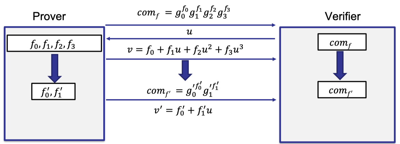
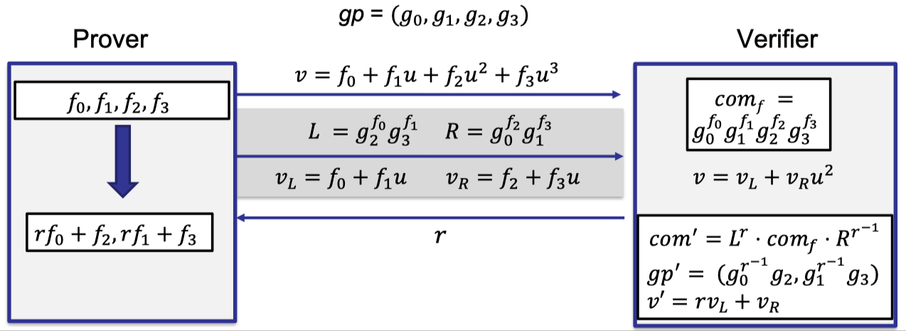
Let’s describe the high-level idea of Bulletproofs reduction using an example of a degree-3 polynomial.

After receiving the commitment to $f$ from the prover, verifier queries at $u$. Prover replies with the evaluation $v$.

The key idea is to reduce the claim of evaluating $v$ at point $u$ for the polynomial $f$ inside the commitment $\text{com}_f$ to a new claim about a new polynomial of only half of the size.

In our example, we reduce the original polynomial of degree 3 to a new polynomial of degree only 1 with only two coefficients $f_0’$ and $f_1’$.

Furthermore, the verifier will receive a new instance of the commitment $\text{com}_{f’}$ to this new polynomial of only half of the size.

Then we keep doing recursively to reduce the polynomial of degree $d/2$ to a new polynomial of degree $d/4,d/8,\dots,$ to a constant degree.

Finally, in the last round, the prover can just send a polynomial of constant size to the verifier directly, and the verifier opens the polynomial and checks the evaluation of the last round is indeed true.

It completes the entire reduction and guarantees that the claim of the evaluation of $v$ for the original polynomial is correct.

The main challenge of the reduction is how to go from the original polynomial to a new polynomial of half of the size.

We can’t have the prover commit to a random polynomial of half of the size without any relationship. Otherwise, the prover can cheat and lie about the evaluation since this new polynomial has no relation to the original polynomial.

It has to check the relationship between the two polynomials.

Let’s elaborate on the details of the reduction.

Prover first sends the evaluation $v=f_0+f_1u+f_2u^2+f_3u^3$ at point $u$.

A common way of reduction for the prover is reducing the polynomial to two polynomials of half of size.

Then prover evaluates these two reduced polynomials at point $u$ to get $v_L=f_0+f_1u$ and $v_R=f_2+f_3u$ such that $v=v_L+v_Ru^2$.

It is safe for the verifier to believe that $v$ is the correct evaluation if and only if $v_L$ and $v_R$ are correctly evaluated for the reduced polynomials.

So prover also commits to the two reduced polynomials with two cross terms $L=g_2^{f_0}g_3^{f_1}$ and $R=g_0^{f_2}g_1^{f_3}$, which uses $g_2,g_3$ as bases to commit to the left reduced polynomial and $g_0,g_1$ to commit to the right reduced polynomial.

As depicted follows, prover sends two commitments $L$ and $R$ and two evaluations $v_L$ and $v_R$ on the two reduced polynomials.

But these two polynomials are actually temporary reduced polynomials.

The actual reduced polynomial is a single polynomial with two coefficients $rf_0+f_2$ and $rf_1+f_3$, which is a randomized linear combination of the original coefficients where the randomness $r$ is sampled by the verifier.

This new claim about this new reduced polynomial actually combines two claims about the old temporary polynomials through randomized linear combinations.

And the claim about the evaluation in the next round is to altered to $v’=rv_L+v_R$.

The only remaining challenge is to generate the commitment of this randomized reduced polynomial.

We can’t let the prover commit $g_0^{rf_0+f_2}g_1^{rf_1+f_3}$ with the original global parameters because the transparent setup doesn’t know the relationship ( defined by $r$ ) between the two polynomials.

In order to address the issue, Bulletproofs proposed a clever design to allow the verifier to compute the new commitment from the old commitments with the help of the commitments to the temporary polynomials.

Recall that $\text{com}_f=g_0^{f_0}g_1^{f_1}g_2^{f_2}\dots g_d^{f_d}$, $L=g_2^{f_0}g_3^{f_1}$ and $R=g_0^{f_2}g_1^{f_3}$. Then verifier can compute the commitment $\text{com}’$ from $L$ and $R$ such that

$$ \begin{aligned} \text{com}' &=L^r\cdot \text{com}_f \cdot R^{r^{-1}} \\ &=g_0^{f_0+r^{-1}f_2}g_2^{rf_0+f_2}\cdot g_1^{f_1+r^{-1}f_3}g_3^{rf_1+f_3} \\ &= (g_0^{r^{-1}}g_2)^{rf_0+f_2} \cdot (g_1^{r^{-1}}g_3)^{rf_1+f_3}\end{aligned} $$

where the global parameter is updated to $gp’=(g_0^{r^{-1}}g_2,g_1^{r^{-1}}g_3)$.

The last equation holds by extracting the common factor to commit to the new polynomial with coefficients $rf_0+f_2$ and $rf_1+f_3$.

And the verifier can compute the new global parameters related to the new commitment, which allows the verifier to check some pairing equations.

Let’s sum up the reduction procedure.

Poly-commitment based on Bulletproofs:

Recurse $\log d$ rounds:

• Eval: (Prover)
  1. Compute $L,R,v_L,v_R$
  2. Receive $r$ from the verifier, reduce $f$ to $f’$ of degree $d/2$
  3. Update the bases $gp’$
• Verify: (Verifier)
  1. Check $v=v_L+v_Ru^{d/2}$
  2. Generate $r$ randomly
  3. Update $\text{com}’=L^r\cdot \text{com}_f\cdot R^{r^{-1}}$, $gp’$, and $v’=rv_L+v_R$

In the last round:

1. The prover sends the constant-size polynomial to the verifier.
2. The verifier checks the commitment and the evaluation is correct.

Note that the above protocol can be rendered non-interactive via Fiat Shamir.

Properties of Bulletproofs

Let’s sum up the properties of poly-commitment based on Bulletproofs.

Properties of Bulletproofs:

• Keygen: $O(d)$, transparent setup!
• Commit: $O(d)$ group exponentiations, $O(1)$ commitment size.
• Eval: $O(d)$ group exponentiations
• Proof size: $O(\log d)$
  In each round, the prover sends 4 elements as proof.
• Verifier time: $O(d)$
  The verifier has to recursively update the global parameters the number of which falls geometrically so the verifier time depends on the first round that is nearly linear in $d$.

Other works

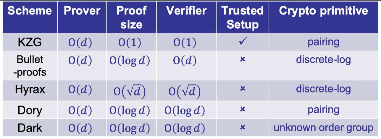
Hyrax

Reference: [Wahby-Tzialla-shelat-Thaler-Walfish’18]

The main drawback of Bulletproofs is the linear verifier time.

Hyrax improves the verifier time to $O(\sqrt{d})$ by representing the coefficients as a 2-D matrix with proof size $O(\sqrt{d})$.

In fact, the product of verifier time and the proof size is linear in $d$ so the proof size can be reduced to $\sqrt[n]{d}$ while the verifier time is $d^{1-1/n}$.

Dory

Reference: [Lee’2021]

Dory improves the verifier time to $O(\log d)$ without any asymptotic overhead on other parts.

It’s a nice improvement over the poly-commitment based on Bulletproofs.

The key idea is delegating the structured verifier computation to the prover using inner pairing product arguments. [BMMTV’2021]

It also improves the prover time to $O(\sqrt{d})$ exponentiations plus $O(d)$ field operations.

Dark

Reference: [Bünz-Fisch-Szepieniec’20]

Dark achieves $O(\log d)$ proof size and verifier time based on the cryptographic primitive of group of unknown order.

---

Let’s end up with a summary of all works mentioned in this lecture.