「Cryptography-ZKP」: Lec7 Poly-commit based on ECC

In this series, I will learn Zero Knowledge Proofs (ZKP) on this MOOC, lectured by Dan Boneh, Shafi Goldwasser, Dawn Song, Justin Thaler and Yupeng Zhang.
Any corrections and advice are welcome. ^ - ^

Topics:

• Poly-commit based on Error-correcting Codes
• Argument for Vector-Matrix Product
  • Proximity Test
  • Consistency Test
• Linear-time encodable code based on expanders
  • Lossless Expander
  • Recursive Encoding with constant relative distance

An important component in the common paradigm for efficient SNARK is the polynomial commitment scheme.

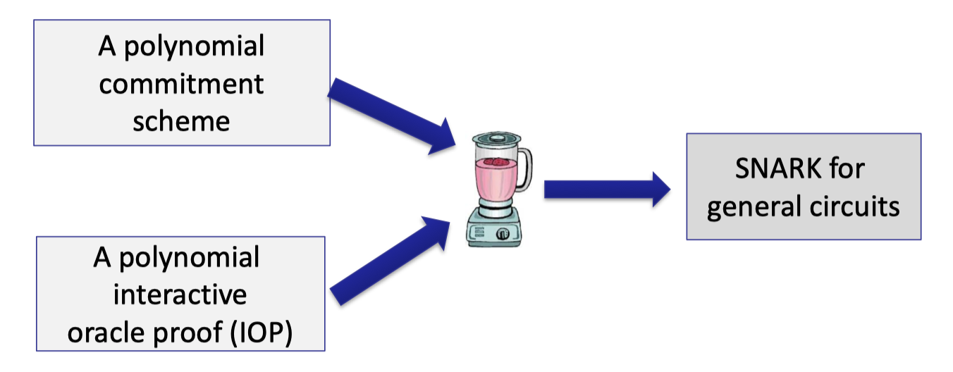
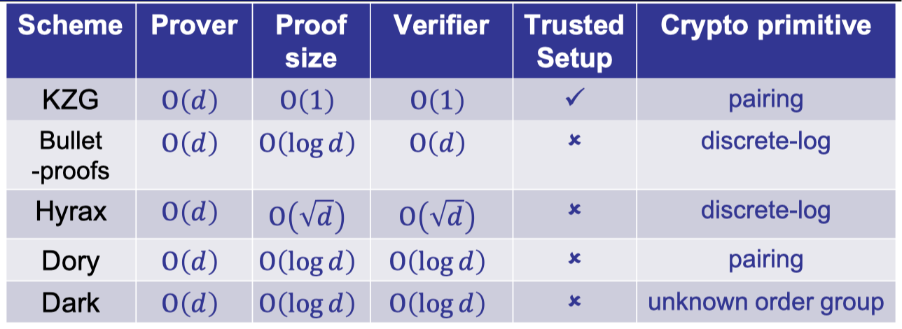
In Lecture 6 we introduced the KZG polynomial commitment based on bilinear pairing and other polynomial commitments based on discrete-log.

It is worth noting that prover time is dependent on $O(d)$ exponentiations, which is not strictly linear-time.

Today we are going to present a new class of polynomial commitments based on error-correcting codes.

Here are the motivations and drawbacks.

Motivations:

• Plausibly post-quantum secure
• No group exponentiations
  Prover only uses hashes, additions and multiplications.
• Small global parameters

Drawbacks:

• Large proof size
• Not homomorphic and hard to aggregate

Background

Error-correcting Code

Let’s briefly introduce the error-correcting code, which is allowed to correct errors.

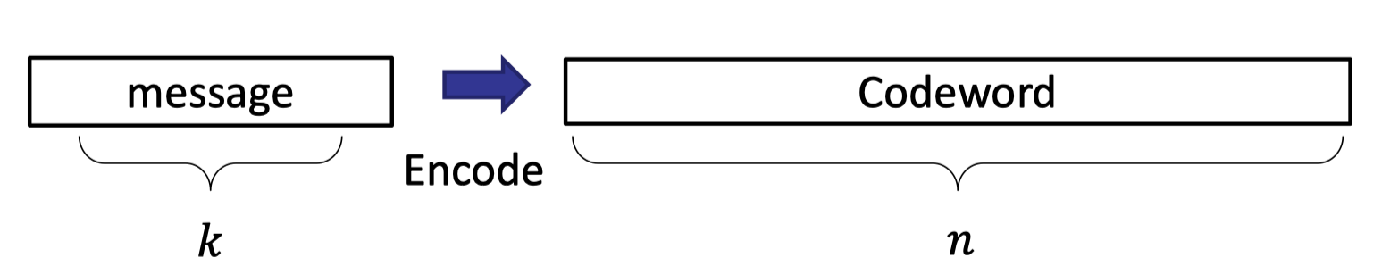
A $[n,k,\Delta]$ code is defined below:

• $Enc(m)$: Encode a message of size $k$ to a codeword of size $n$.
• Minimum distance (Hamming distance) between any two codewords is $\Delta$.

Note that we omit the alphabet $\Sigma$ (binary or field) here, which is another important parameter in code.

A simple example is the repetition code, which just repeat each symbol three times.

Consider the binary alphabet with $k=2$ and $n=6$.

The codewords are Enc(00)=000000, Enc(01)=000111, Enc(10)=111000 and Enc(11)=111111 with minimum distance $\Delta=3$.

This repetition code with minimum distance $\Delta=3$ can correct 1 error duting the transmission.

E.g., suppose the transmission can induce at most 1 error, then the message 010111 received from the sender can be decoded to 01.

It is worth mentioning that we are going to build poly-commit using error-correcting code without efficient decoding algorithm.

The truth is that we don’t use the decoding algorithm at all.

We define rate and relative distance over a $[n,k,\Delta]$ code.

The rate $\frac{k}{n}$ represents the ratio of the minimal message in the codeword of size $n$. We want the rate close to 1.

The relative distance $\frac{\Delta}{n}$ represents the ratio of the different locations between any two codewords.

E.g., repetition code with rate $\frac 1 a$ repeats each symbol $a$ times with $n=ak$, and has $\Delta=a$ and relative distance $\frac 1 k$.

We want rate and relative distance as big as possible, but increasing rate could decrease the relative distance.

The trade-off between the rate and the distance of a code is well studied in code theory.

Linear Code

The most common type of code is linear code.

An important property is any linear combination of codewords is also a codeword.

It is equivalent to say that encoding can always be represented as vector-matrix multiplication between $m$ (of size $k$) and the generator matrix (of size $k\times n$).

Moreover, the minimum (Hamming) distance is the same as the codeword with the least number of non-zeros (weight).

(The weight of a codeword indicats the number of non-zeros.)

The subtraction of any two codewords is also a codeword so the number of the different locations directly implies the weight of another non-zero codeword.

Reed-Solomon Code

A classical construction of linear code is Reed-Solomon Code.

It encodes messages in $\mathbb{F}_p^k$ to codewords in $\mathbb{F}_p^n$.

The idea of encoding is veiwing the message of size $k$ as a unique degree $k-1$ univariate polynomial and the codeword is the evaluations at $n$ points.

It treats each symbol of the message as an evaluation at a pre-defined point so the polynomial can be uniquely defined by interpolation on the fixed set of public points.

Then we can evaluate $n$ pre-defined public points as the codeword. E.g., $(\omega,\omega^2,\dots, \omega^n)$ for $n$-th root-of-unity $\omega^n=1 \mod p$.

The minimal distance is $\Delta=n-k+1$ (indicating the least number of non-zeros) since a degree $k-1$ polynomial has at most $k-1$ roots (indicating the most number of zero evaluations).

E.g., when $n=2k$, rate is $\frac 1 2$ and relative distance is $\frac 1 2$.

It is pretty good in practice and is almost the best we can achieve.

RS code is a linear code that the encoding algorithm can be represented as vector-matrix multiplication where the vector is the message and the generator matrix can be derived from Fourier matrix.

The encoding time is $O(n\log n)$ using the fast Fourier transform (FFT).

Poly-commit based on error-correcting codes

Recall the polynomial commitment scheme we discussed in previous lectures.

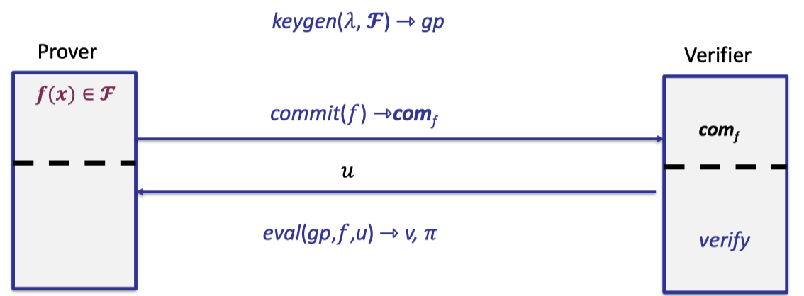
1. keygen generates global parameters for $\mathbb{F}_p^{(\le d)}$.
2. Prover commits to a univariate polynomial of degree $\le d$ .
3. Later verifier requests to evaluate at point $u$.
4. Prover opens $v$ with proof that $v=f(u)$ and $f\in \mathbb{F}_p^{(\le d)}$.

Reduce PCS to Vec-Max Product

In the poly-commit based on error-correcting codes, we write the polynomial coefficients in a matrix of size $\sqrt{d}$ by $\sqrt{d}$.

For simplicity, we assume $d$ is an exact power.

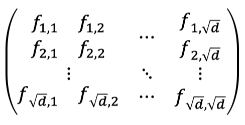
Note that the vectorization of the above matrix forms the original vector of polynomial coefficients, that is:

$$ [f_{1,1},f_{2,1},\dots, f_{\sqrt{d},1},\dots,f_{1,\sqrt{d}},\dots,f_{\sqrt{d},\sqrt{d}}]^{T} $$

Hence, the polynomial behind the matrix can be written with two indices:

$$ f(u)=\sum_{i=1}^{\sqrt{d}}\sum_{j=1}^{\sqrt{d}} f_{i,j}u^{i-1+(j-1)\sqrt{d}} $$

Then the evaluation of $f(u)$ can be viewed as two steps as follows.

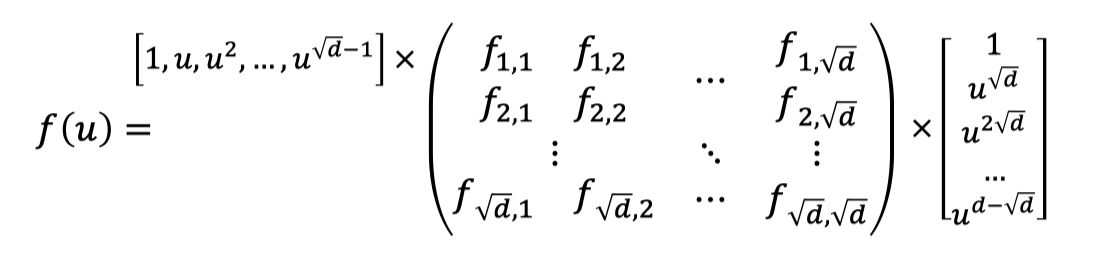
Two steps of evaluation:

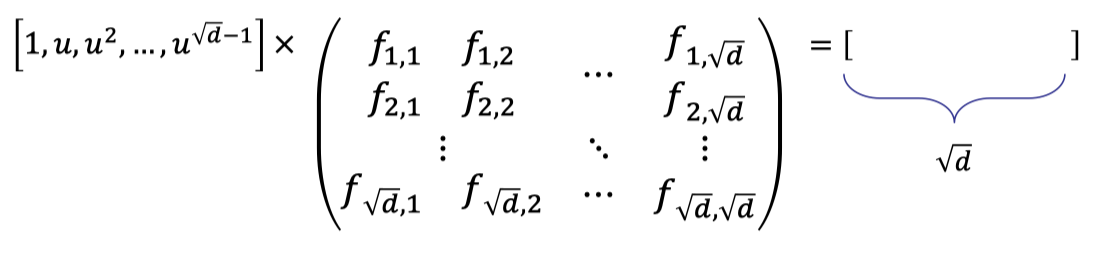
1. (Vecor-Matrix Product) Multiply a vector defined by point $u$ with the matrix of coefficients to get a vector of size $\sqrt{d}$.

   

2. (Inner Product) Multiply the vector of size $\sqrt{d}$ with another vector defined by point $u$ to obtain the final evaluation.

With this nice observation, we actually reduce the poly-commit to an argument for vector-matrix product.

Roughly speaking, prover can only evaluate the first step and sends a vector of size $\sqrt{d}$ as proof.

Verifier checks whether the Vec-Mat product is correct using proof system and evaluates the second step locally, which is an inner product of the Vec-Mat product and the vector defined by point $u$.

As a result, the argument for Vec-Mat product gives us a polynomial commitment with $\sqrt{d}$ proof size.

Argument for Vec-Mat Product

Now our goal is to design a scheme to test the Vec-Mat product without sending the matrix directly.

Commit

As usual, we need to commit to the polynomial.

Here we instead commit to an encoded matrix defined by the polynomial.

We first use a linear code to encode the original matrix defined by the coefficients of polynomial.

Concretely speaking, we encode each row with a linear code to compute an encoded matrix of size $\sqrt{d}\times n$ where $n$ is the size of the codeword.

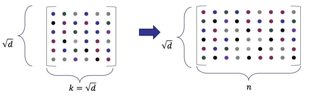
We will use a linear code with constant rate so that the size of the encoded matrix is asymptotical to $d$.

Then we can commit to each column of the encoded matrix using Merkle tree.

Recall the Merkle tree commitment introduced in [Lecture 4].

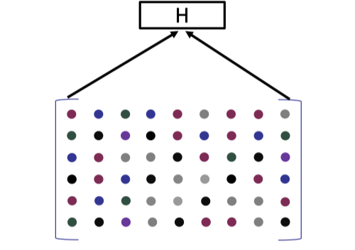
The root hash is served as the commitment to the encoded matrix.

Then verifier can request to open each column individually and checks whether the opened column is altered.

It is worth noting that the key generation for this Merkle tree commitment is only sampling a hash function, resulting in a constant size global parameters with no trusted setup.

Eval and Verify

We actually perform the evaluation together with verification.

It consists of two tests, proximity test and consistency check.

We fisrt consider how a malicious prover could cheat in the commitment.

A malicious prover can commit to a matrix of inappropriate size but it can be recognized easily by the Merkle tree proof.

A malicious prover can commit to an abitrary matrix of specified size in which each row is not a valid codeword.

E.g., a valid RS code is a vector of evaluations of a polynomial specified by the message.

Hence, verifier uses the proxomity test to test if the committed matrix indeed consists of $\sqrt{d}$ codewords.

Having checked this proximity test, verifier is convinced that the committed matrix is nearly close to the encoded matrix defined by the original matrix of coefficients.

Then verifier can move to the consistency check to compute (and verifiy) the actual evaluation.

Step1: Proximity Test

Ligero [AHIV’2017] and [BCGGHJ’2017] are two independent works to introduce the proximity test.
Ligero proposed the so-called interleaved test using Reed-Solomon code with quasi-linear prover time.
[BCGGHJ’2017] instead used a linear-time encodable code to build the ideal linear commitment model, which is the first work to build SNARK with strictly linear prover time.
Note that the proximity test in these two works are proposed to build general-purpose SNARKs. Here we use it to build poly-commit as a specified protocol.

Ligero [AHIV’2017] and [BCGGHJ’2017] are two independent works to introduce the proximity test.

Ligero proposed the so-called interleaved test using Reed-Solomon code with quasi-linear prover time.

[BCGGHJ’2017] instead used a linear-time encodable code to build the ideal linear commitment model, which is the first work to build SNARK with strictly linear prover time.

Note that the proximity test in these two works are proposed to build general-purpose SNARKs. Here we use it to build poly-commit as a specified protocol.

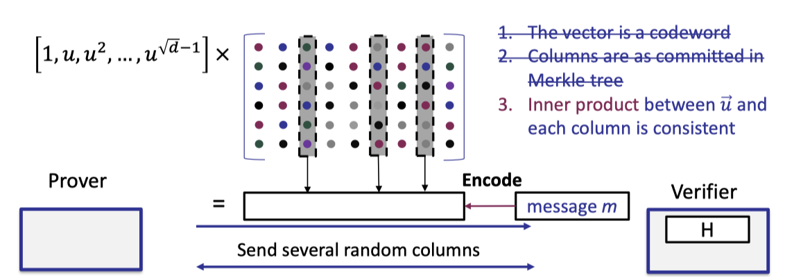
We first present the description of the proximity test as below.

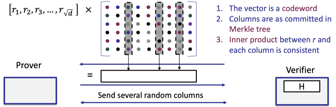
1. Verifier samples a random vector $r$ of size $\sqrt{d}$ and sends it to prover.
2. Prover returns the vector-matrix product of the random vector $r$ and the encoded matrix.
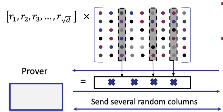
3. Verifier requests to open several random columns and prover reveals them with Merkle tree proof.
4. Verifier performs 3 checks
   1. The returned vector is a codeword
   2. The opened columns are consistent with the committed Merkle tree.
   3. The inner product between $r$ and the opened column is consistent with the corresponding element of the returned vector.

The completeness is evident.

The vec-mat product computed by the honest prover is indeed the linear combination of rows (codewords) specified by the random vector chosen by the verifier.

Recall the propery of the linear codes that a linear combination of codewords is a codeword.

So these 3 checks will be passed by verifier.

Let’s intuitively give the proof of soundness.

Assume for the contradiction that the malicious prover commits to a fake matrix, and computes the vec-mat product by this fake matrix.

Soundness (Intuition):

• If the vector is correctly computed, under our assumption, the product is not a codeword. → check 1 will be failed.
• If the vector is false meaning that the prover just returns an arbitrary codeword, there are many different locations from the correct answer.
  • By check 2, columns are as committed.
  • Probability of passing check 3 is extreamly small.

Let’s discuss the second case where the vector sent by the prover is false and $w=r^TC$ denotes the correct answer.

In the formal proof for soundness: [AHIV’2017], it defines a parameter $e<\frac{\Delta}{4}$, which is related to the minimal distance $\Delta$, to measure the distance between the committed matrix and the codeword space.

Concretely speaking, $e$ measures the minimal distance between any row (of the committed matrix) and any codeword (in the codeword space).

If the committed (fake) matrix is $e$-far from any codeword for $e<\frac{\Delta}{4}$, then the probability that the vec-mat product $w=r^T C$ is $e$-close to any codeword is $\le \frac{e+1}{\mathbb{F}}$, which is extreamly small.

$$ \operatorname{Pr}[w=r^TC\text{ is }e\text{-close to any codeword}]\le \frac{e+1}{\mathbb{F}} $$

Then we can rule out this case, and the remaining case is that the correct answer $w=r^TC$ is $e$-far from any codeword.

Under this condition, we know there are at least $e$ different positions between the codeword sent by prover and the correct answer $w$.

Then the probability that check 3 is true for $t$ random columns is bounded by $(1-\frac e n)^t$ where $\frac e n$ is constant for the linear code with constant relative distance, e.g. RS code.

$$ \operatorname{Pr}[\text{check 3 is true for }t \text{ random columns}] \le (1-\frac{e}{n})^t $$

Hence, soundness probability can be reduced to negligible probability. That’s why we want linear codes with constant relative distance.

Optimization for Proximity Test

There is one optimization for the proximity test.

Instead of sending the codeword, prover can send the message behind the codeword to verifier.

Note that the message is computed by the random vector and the original matrix defined by the polynomial coefficients.

Then verifier can encode the message to obtain the corresponding codeword that is supposed to be sent by prover.

This nice optimization reduces the proof size from $n$ to $k$.

Moreover, there is no need for verifier to perform the first check explicitly that the vector is a codeword since the encoding is done by the verifier.

We depict the optimized proximity test as below.

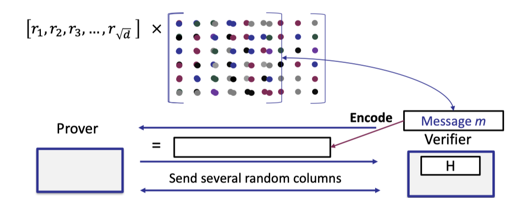
1. Verifier samples a random vector $r$ of size $\sqrt{d}$ and sends it to prover.
2. Prover returns the vector-matrix product of the random vector $r$ and the original matrix of coefficients.
3. Verifier encodes the message to compute the codeword.
4. Verifier requests to open several random columns and prover reveals them with Merkle tree proof.
5. Verifier performs 2 checks
   1. The returned vector is a codeword
   2. The opened columns are consistent with the committed Merkle tree.
   3. The inner product between $r$ and the opened column is consistent with the corresponding element of the returned vector.

Step2: Consistency Check

With the proximity test, the verifier knows the committed matrix is close to an encoded matrix with overwhelming probability.

Next we can perform the consistency check to really test the evaluation of vec-mat product between the vector defined by point $u$ and the original matrix of size $\sqrt{d}\times \sqrt{d}$.

The consistency check is almost the same as the proximity test with the optimization mentioned above excetp that the vector is defined by point $u$ rather than a random vector $r$.

Likewise, the verifier encodes the message to compute the codeword so the first check can be removed.

Futhermore, the verifier can use the same opened columns in the proximity test to perform the third check.

The cosistency check is depicted as below where the first two checks can be removed.

Knowledge Soundness (Intuition):

In the consistency test, we actually need to prove the knowledge soundness.

By the proximity test, the committed matrix $C$ is close to an encoded matrix that can be uniquely decoded to a matrix $F$ defined by polynomial coefficients.

Intuitively speaking, there exists an extractor that extracts $F$ by Merkle tree commitment and decoding $C$, s.t. $\vec{u}\times F=m$ with probability $1-\epsilon$.

Summary

To put everything together, the poly-commit scheme based on linear code is described as below.

PCS based on Linear Code:

• Keygen: sample a hash function
• Commit:
  1. encode the coefficient matrix $F$ of $f$ row-wise with a linear code
  2. compute the Merkle tree commitment col-wise
• Eval and Verify:
  • Proximity test: random linear combination of all rows, check its consistency with $t$ random columns
  • Consistency test: compute $\vec{u}\times F=m$, encode $m$ and check its consistency with $t$ random columns
  • Evaluate $f(u)=<m,u’>$ by verifier where $u’$ is another vector defined by point $u$.

An important thing to point out is that the proximity test is necessary for evaluation and verification although it is almost the same as the consistency test.

Suppose we only perform the consistency test, then the verifier checks consistency of the inner-product of vector $\vec{u}$ and the random columns.

But it dose not work since vector $\vec{u}$ is defined in a very structured way.

Intuitively speaking, it has to use random challenges chosen by the verifier to guarantee the consistency.

Properties:

• Keygen: $O(1)$, transparent setup with constant size $gp$.
• Commit:
  • Encoding: $O(d\log d)$ field multiplications using RS code, $O(d)$ using linear-time encodable codes.
  • Merkle tree: $O(d)$ hashes, $O(1)$ commitment size.
• Eval: $O(d)$ field multiplications
• Proof size: $O(\sqrt{d})$ (several vectors of size $\sqrt{d}$ )
• Verifier time: $O(\sqrt{d})$

Look at the concrete performance in [GLSTW’21] with degree $d=2^{25}$ and linear-time encodable code.

• Commit: 36s
• Eval: 3.2s
• Proof size: 49MB
• Verifier time: 0.7s

It is excellent in practice and significantly faster than PCS based on pairing or discrete-log (such as KZG, Bulletproofs) because it only uses linear operations without any exponentiations.

Related Works

Let’s disscuss the following up-to-date works based on error-correcting codes.

• [Bootle-Chiesa-Groth’20]

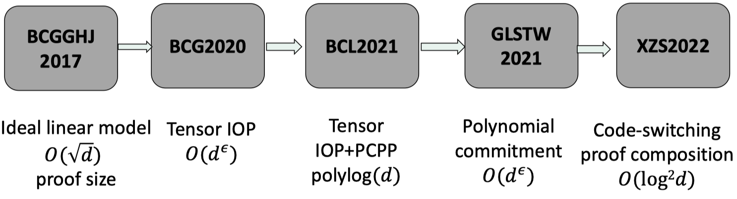
It proposed the tensor query IOP $<f,(\vec{u}\otimes \vec{u}’)>$, which evaluates inner-product of vector $f$ of size $\sqrt{d}$ and another vector generated by tensor product between two sub-vectors of size $\sqrt{d}$. (dimentsion 2)

Note that this IOP only works for the product of specific form.

Moreover, it generalizes to multiple dimentsions and performs the proximity test and consistency test dimension by dimension with smaller proof size $O(n^\epsilon)$ for constant $\epsilon<1$.

• Brakedown [GLSTW’21]

This work proposed the polynomial commitment based on tensor query.

As described above, we don’t use decoding algorithm at all in the poly-commit. The prover just sends the message and the verifier encodes the message to get the corresponding codeword. It gives relaxation on the design of the poly-commit which allows to use linear codes without efficient decoding algorithm.

Unfortunately, when we prove the knowledge soundness, it has to extract the matrix of polynomial coefficients from the committed encoded matrix in which the efficient decoding is required. If the decoding algorithm is not efficient, the extractor is not polynomial as well.

Back to this work, the another contribution is showing an alternative way to prove knowledge soundness without efficient decoding algorithm.

As a result, it enables us to build poly-commit using any linear codes without efficient decoding algorithm.

• [Bootle-Chiesa-Liu’21]

It improves proof size to $\text{poly}\log (n)$ with a proof composition of tensor IOP and PCP of proximity. [Mie’09]

• Orion [Xie-Zhang-Song’22]

It improves the proof size to $O(\log^2 n)$ with a proof composition of the code-switching technique [Ron-Zewi-Rothblum’20]

Concretely, the proof size is 5.7MB for $d=2^{25}$, which is quite large in practice.

Linear-time encodable code based on expanders

It is noteworthy that the following line of works all build SNARKs with linear prover using the linear-time encodable code with constant relative distance.

In the last segment, we are going to present the construction of linear-time encodable code based on expanders.

Linear-time encodable code is proposed by [Spielman’96] and generalized from binary to field by [Druk-Ishai’14], which relies on the expander graph.

Expander Graph

Look at the following bipartite graph where each node on the left set has 3 outgoing edges connecting to the nodes on the right edges and every two nodes on the left set connect at least 5 nodes on the right set.

Bipartite Graph (from wiki)
A bipartite graph is a graph whose vertices can be divided into two disjoint and independent sets U and V, that is, every edge connects a vertex in U to one in V. Vertex sets U and V are usually called the parts of the graph.

It is a good expander since every two nodes on the left set have at most 6 outgoing edges.

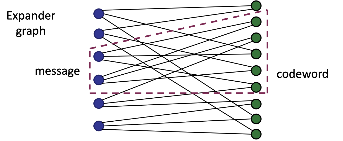
In terms of encoding, consider the left nodes as message where each symbol is put on a node and the right nodes is the codeword.

The encoding of the message is to compute for each right-side node the sum of nodes connected from the left set, which can be represented as the vector-matrix multiplication between the message and the adjacent matrix of the graph so it is a linear code.

A nature question is why we need such an expander graph to achieve linear codes with a good relative distance.

Intuitively speaking, with such a good expander, even a single non-zero node on the left set can be expanded to many non-zero nodes on the right set, that is, it amplies the number of non-zeros (weight) from the message to the codeword, enabling us to achieve good relative distance.

Lossless Expander

Note that the relative distance in the above simple example is not constant.

We are going to describe the lossless expander in a formal way.

Let $|L|$ denote the number of left nodes and the number of the right nodes is $\alpha |L|$ for a constant $\alpha\in (0,1)$.

The degree of a left node is denoted by $g$.

Consider a good (almost perfect) expander that for every subset $S$ of nodes on the left, the number of neighers $|\Tau(S)|=g|S|$ for $|S|\le \frac{\alpha |L|}{g}$, which is bounded by the number of right nodes.

But it is too good to achieve.

We need to relax the equality and the boundary.

Lossless Expander:

For every subset $S$ of nodes on the left, the number of neighbors $|\Tau(S)|\ge (1-\beta)g|S|$ for $|S|\le \frac{\delta |L|}{g}$.( $\beta\rightarrow 0$, $\delta \rightarrow \alpha$ )

Likewise, the encoding on the lossless expander is to sum up the connected nodes from the left nodes for each right node to compute the codeword.

Recursive Encoding

Then we move to the construction of linear-time encodable codes, which uses the recursive encoding with the lossless expander.

The encoding algorithm is depicted as below.

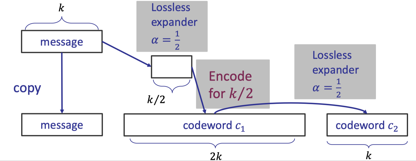
Let’s elaborate on the detailed procedure of encoding a message $m$ of size $k$ to a codeword of size $4k$ with rate $1/4$.

Recursive Encoding:

1. Copy the message as the first part of the final codeword.
2. Apply the lossless expander with $\alpha=\frac 1 2$ to compute the codeword $m_1$ of size $k/2$.
3. Assume we already had an encoding algorithm for message $m_1$ of size $k/2$ with rate $1/4$ and good relative distance $\Delta$, then we apply it to compute the codeword $c_1$ of size $2k$ as the second part of the final codeword.
4. Apply another lossless expander with $\alpha =\frac 1 2$ for messages of size $2k$ to compute the codeword $c_2$ of size $k$ as the third part.
5. The final codeword is the concatenation $c=m|| c_1||c_2$

The remaining thing is how we get the encoding algorithm for messages of size $k/2$ with rate $1/4$ and good relative distance.

That’s exactly the recursiving encoding that we just use the entire encoding algorithm for the message of size $k/2$.

Hence, we repeate the entire encoding algorithm in recursion from $k/2,k/4,\dots$ until a constant size.

Note that the lossless expanders used in each iteration are different since the size of message are different.

Finally we can use any code with good distance for a constant-size message. E.g., Reed-Solomon code.

Distance of the Code

The recursive way of encoding enables to achieve a constant relative distance:

$$ \Delta'=\min \{\Delta,\frac{\delta}{4g}\} $$

where $\Delta$ is the relative distance of the code used in the middle from $k/2$ to $2k$ and $\frac{\delta}{4g}$ depends on the expander graph.

Proof of relative distance (case by case): [Druk-Ishai’14]

1. If weight of $m$ is larger than $4k\Delta’$, then the relative distance is larger than $\frac{4k\Delta’}{4k}=\Delta’$.
   → Done. It means that for all messages with large weight, we automatically get codewords with large weight.
2. If weight of $m\le 4k\Delta'\le \frac{\delta k}{g}$, the condition of the first lossless expander holds. (since $\Delta'\le \frac{\delta}{4g}$ )
   1. Let $S$ be the set of non-zero nodes in $m$, then we have $|\Tau(S)|\ge (1-\beta)g|S|$.
   2. We can set $g\ge 10$ and $\beta < 0.1$, then at least $(1-2\beta)g|S| > 8|S|>0$ vertices in Hamming ball have a unique neighbor in $S$.
   3. Hence, $m_1$ (the output of this lossless expander) is non-zero.
   4. After applying the encoding for $m_1$ of size $k/2$ with relative distance $\Delta$, the wight of $c_1$ $\ge 2k\Delta\ge 2k\Delta’$.
      (The second inequality holds by the definition of min).
3. If the weight of $c_1$ is larger than $4k\Delta’$, then the relative distance is larger than $\Delta’$.
   →Done
4. Else, weight of $c_1$ is $\le 4k\Delta’<\frac{\delta2k}{g}$, the condition of the second lossless expander holds.
   1. Let $S’$ be the set of non-zero nodes in $c_1$, then we can show the weight of $c_2$ is at least $|\Tau(S’)|\ge (1-\beta)g|S’|>8|S’|>16k\Delta’ >(4k)\Delta’$.

Sampling of the Lossless Expander

With lossless expander, we can build the linear-time encodable codes with constant relative distance.

The last piece of the puzzle is how to construct the lossless expander.

[Capalbo-Reingold-Vadhan-Widgerson’2002] proposed an explicit construction of lossless expander.

Note that being explicit is deterministic.

Unfortunately, it has large hidden constant so the concrete efficiency is not good.

An alternative way is random sampling since a random graph is supposed to have good expansion.

Since the sample space is polynomial, there is a $1/\text{poly}(n)$ failure probability instead of negligible probability.

Improvements of the Code

• Brakedown [GLSTW’21]

Instead of the plain summations when encoding, it uses random summations, which assign a random weight for each edge and performs the weighted summation, to significantly boost the distance.

• Orion [Xie-Zhang-Song’22]

It proposes an expander testing with a negligible failure probability via maximum density of the graph.

---

Let’s sum up the pros and cons of the polynomial commitment (and SNARK) based on linear code.

• Pros
  • Transparent setup: $O(1)$
  • Commit and Prover time: $O(d)$ field additions and multiplications
  • Plausibly post-quantum secure
  • Field agnostic
    It means that we can use any field.
• Cons
  • Proof size: $O(\sqrt{d})$, MBs